Notes on Stochastic Processes (Joe Chang)
Ch. 1 – Markov Chains
1.1 Specifying and Simulating a Markov Chain
to specify a Markov chain, we need to know its
- state space , a finite or countable set of states—values the random variables may take on
- initial distribution , the probability distribution of the Markov chain at time .
- for each state , , the probability the Markov chain starts in state we can also think of are a vector whose -th entry is
- probability transition matrix
- if has states, then is
- or is the probability that the chain will transition to from : .
- rows sum to 1 (think: from state , we are in row , and there must be probability 1 of going to any next state )
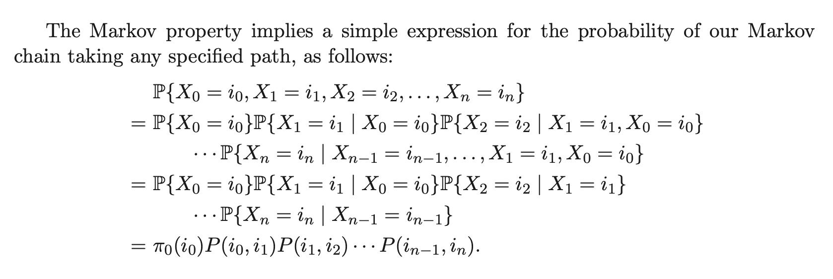
1.2 The Markov Property
a process satisfies the Markov property if
for all and all .
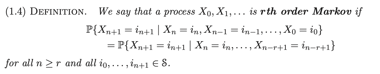
(i.e., dependent on the last r states)
1.3 Matrices
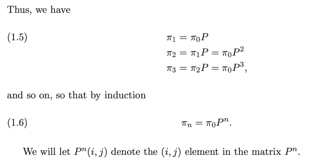
recall from 1.1. let denote the distribution of the chain at time analogously, . consider both as row vectors.
suppose that the state space is finite: . by LOTP,
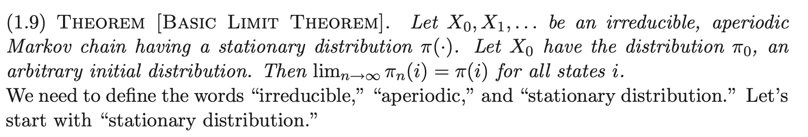
1.4 Basic Limit Theorem of Markov Chains
1.5 Stationary Distribution
stationary distribution amounts to saying is satisfied, i.e.,
for all .
a Markov chain might have no stationary distribution, one stationary distribution, or infinitely many stationary distributions.
for subsets of the state space, define the probability flux from set into as
1.6 Irreducibility, Periodicity, Recurrence
Use as shorthand for , and same for .
Accessibility: for two states , we say that is accessible from if it is possible for the chain ever to visit state if the chain starts in state :
Equivalently,
Communication: we say communicates with if is accessible from and is accessible from .
Irreducibility: the Markov chain is irreducible if all pairs of states communicate.
The relation “communicates with” is an equivalence relation; hence, the states space can be partitioned into “communicating classes” or “classes.”
–
The Basic Limit Theorem requires irreducibility and aperiodicity (see 1.5). Trivial examples why:
- Irreducibility: takes . Then holds for all , i.e., does not approach a limit independent of .
- Aperiodicity: same , take . If, for example, alternates with even and odd , and does not converge to anything.
–
Period: Given a Markov chain , define the period of a state to be the greatest common divisor
THEOREM: if the states and communicate, then .
The period of a state is a “class property.” In particular, all states in an irreducible Markov chain have the same period. Thus, we can speak of the period of a Markov chain if the Markov chain is irreducible.
An irreducible Markov chain is aperiodic if its period is , and periodic otherwise. (A sufficient but not necessary condition for an irreducible chain to be aperiodic is that there exists a state such that .)
–
One more concept for the Basic Limit Theorem: recurrence. We will begin with showing recurrence, then showing that it is a class property. In particular, in an irreducible Markov chain, etiher all states are recurrent OR all states are transient.
The idea of recurrence: a state is recurrent if, starting from the state at time 0, the chain is sure to return to eventually. More precisely, define the first hitting time of the state i by
Recurrence: the state is recurrent if . If is not recurrent, it is called transient.
(note that accessibility could be defined: for distinct states , is accessible from iff .)
THEOREM: Let be a recurrent state, and suppose that is accessible from . Then all of the following hold:
- The state is recurrent
–
We use the notation for the total number of visits of the Markov chain to the state :
THEOREM: The state is recurrent iff
COROLLARY: If is transient, then for all states .
–
Introducing stationary distributions.
PROP: Suppose a Markov chain has a stationary distribution . If the state is transient, then .
COROLLARY: If an irreducible Markov chain has a stationary distribution, then the chain is recurrent.
Note that the converse for the above is not true. There are irreducible, recurrent Markov chains that do not have stationary distributions. For example, the simple symmetric random walk on the integers in one dimension is irreducible and recurrent but does not have a stationary distribution. By recurrence we have , but also . The name for this kind of recurrence is null recurrence, i.e., a state is null recurrent if it is recurrent and . Otherwise, a recurrent state is positive recurrent, where .
Positive recurrence is also a class property: if a chain is irreducible, the chain is either transient, null recurrent, or positive recurrent. In fact, an irreducible chain has a stationary distribution iff it is positive recurrent.
1.7 Coupling
Example of coupling technique: consider a random graph on a given finite set of nodes, in which each pair of nodes is joined by an edge independently with probability . We could simulate a random graph as follows: for each pair of nodes generate a random number , and join nodes and with an edge if .
How do we show that the probability of the resulting graph being connected is nondecreasing in , i.e., show that for ,
We could try to find an explicit function for the probability in terms of , which seems inefficient. How to formalize the intuition that this seems obvious?
An idea: show that corresponding events are ordered, i.e., if then .
Let’s make 2 events by making 2 random graphs, on the same set of nodes. is constructed by having each possible edge appear with prob , and for , each edge present with prob We can do this by using two sets of random variables: for the first and second graph, respectively. Is it true that
No, since the two sets of r.v.s are independently generated.
A change: use the same random numbers for each graph. Then
becomes true. This establishes monotonicity of the probability being connected.
Conclusion: what characterizes a coupling argument? Generally, we show that the same set of random variables can be used to construct two different objects about which we want to make a probabilistic statement.
1.8 Proof of Basic Limit Theorem
The Basic Limit Theorem says that if an irreducible, aperiodic Markov chain has a stationary distribution , then for each initial distirbution , as we have for all states .
(Note the wording “a stationary distribution”: assuming BLT true implies that an irreducible and aperiodic Markov chain cannot have two different stationary distributions)
Equivalently, let’s define a distance between probability distributions, called “total variation distance:”
DEFINITION: Let and be two probability distributions on the set . Then the total variation distance is defined by
PROP: The total variation distance may also be expressed in the alternative forms
We now introduce the coupling method. Let be a Markov chain with the same probability transition matrix as , but let have the initial distribution and have the initial distribution . Note that is a stationary Markov chain with distribution for all . Let the chain be independent of the chain.
We want to show that, for large , the probabilistic behavior of is close to that of .
Define the coupling time to be the first time at which :
LEMMA: For all n we have
Hence we need only show that , or equivalently, that
Consider the bivariate chain is clearly a Markov chain on the state space . Since the and chains are independent, the probability transition matrix of chain can be written
has stationary distribution
We want to show So, in terms of the chain, we want to show that with probability one, the chain hits the “diagonal” in in finite time. To do this, it is sufficient to show that the chain is irreducible and recurrent.
This is where we use aperiodicity.
LEMMA: Sps is a set of positive integers closed under addition, with gcd one. Then there exists an integer s.t. for all .
Let and recall the assumption that the chain is aperiodic. Since the set is closed under addition, and, from aperiodicity, has greatest common divisor , we can use the previous lemma. So for all sufficiently large . From this, for any , since irreducibility implies for some m, it follows that for all sufficiently large .
Now we show irreducibility. Let . It is sufficient to show that for some . By the assumed independence of and , we have
which (by the previous argument) is positive for all sufficiently large , so we are done.
1.9 SLLN for Markov Chains
The usual Strong Law of Large Numbers for iid random variables says that if are iid with mean , then
We will do a generalization of this result for Markov chains: the fraction of times a Markov chain occupies state converges to a limit.
Although the successive states of a Markov chain are not independent, certain features of a Markov chain are independent of each other. Here we will use the idea that the path of the chain consists of a succession of independent “cycles,” the segments of the path between successive visits to a recurrent state. This independence allows us to use the LLN that we already know.
THEOREM: Let be a Markov chain starting in the state , and suppose that the state communictes with another state . The limiting fraction of time that the chain spends in state is . That is,
In the proof of the previous theorem, we define as the number of visits made to state made by , i.e.,
Using the Bounded Convergence Theorem,
we have the following:
COROLLARY: For an irreducible Markov chain, we have
for all states and .
Consider an irreducible, aperiodic Markov chain haing a stationary distribution . From the Basic Limit Theorem, we know that as . Notice also that if a sequence of numbers converges to a limit, then the sequence of Cesaro averages converges to the same limit, i.e., if as , then as . However, the previous Corollary shows the Cesaro averages of 's converge to . So, we must have
In fact, aperiodicity is not needed for this conclusion:
THEOREM: An irreducible, positive recurrent Markov chain has a unique stationary distribution given by
1.10 Exercises
Ch. 2 – Markov Chains: Examples & Applications
2.1 Branching Processes
Motivating example: the branching process model was formulated by Galton, who was interested in the survival and extinction of family names.
Suppose children inherit their fathers’ names, so we need only to keep track of fathers and sons. Consider a male who is the only member of his generation to have a given family name, so that the responsibility of keeping the family name alive falls upon him–if his line of male descendants terminates, so does the family name.
Suppose for simplicity that each male has probability of producing no sons, of producing 1 son, and so on.
What is the probability that the family name eventually becomes extinct?
To formalize this, let:
- the number of males in generation
- Start with
- If , write , where is the number of sons fathered by the -th man in generation
- Assume the r.v.s are iid with probability mass function
- Hence for .
- To avoid trivial cases, assume and .
We are interested in the extinction probability .
is a Markov chain. State 0 is absorbing. So, for each , since , the state must be transient.
Consequently, with probability 1, each state is visited only a finite number of times. So, with probability 1, the chain must get absorbed at 0 or approach .
We can obtain an equation for by conditioning on what happens at the first step of the chain:
Since the males all have sons independently,
Thus, we have
For each distribution there is a corresponding function of denoted . So the extinction probability is a fixed point of .
is the probability generating function of the probability mass funcion . The first two derivatives are
for Since these are positive, the function is strictly increasing and convex on Also note that . Finally, , where , the expected number of sons for each male.
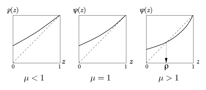
Since , there is always a trivial solution at . When , this trivial solution is the only solution, so .
When , we define to be the smaller solution of . Since , we know that must be either or 1. We want to show that .
Defining , observe that as ,
Therefore, to rule out , it is sufficient to prove that
By induction, observe . Next,
i.e., Since is increasing and by the induction hypothesis , we have that
So is bounded by for all non negative , which proves . Hence there is a non negative probability that the family name goes on forever.
2.2 Time Reversibility
2.3 More on Time Reversibility: A Tandem Queue Model
2.4 The Metropolis Method
2.5 Simulated Annealing
2.6 Ergodicity Concepts
In this section we focus on a time-inhomogeneous Markov chain on a countably infinite state space .
Let denote the probability transition matrix governing the transition from to , i.e.,
For , define s.t.
DEFINITION: is strongly ergodic if there exists a probability distribution on such that
DEFINITION: is weakly ergodic if there exists a probability distribution on such that
We can understand weak ergodicity somewhat as a “loss of memory concept.” It says that at a large enough time , the chain has nearly forgotten its state at time , in the sense that the distribution at time would be nearly the same no matter waht the state was at time . However, there is no requirement that the distribution be converging to anything as . The concept that incorporates convergence in addition to loss of memory is strong ergodicity.
2.6.1 The Ergodic Coefficient
For a probability transition matrix the ergodic coefficient of is defined to be the maximum total variation distance between pairs of rows of , that is,
DEFINITION: The ergodic coefficient of a probability transition matrix is
The basic idea is that being small is “good” for ergodicity. For example, in the extreme case of , all the rows of are identical, so would cause a Markov chain to lose its memory completely in just one step: does not depend on .
LEMMA: for probability transition matrices .
2.6.2 Sufficient Conditions for Weak and Strong Ergodicity
Sufficient conditions are given in the next two propositions:
PROP: If there exist such that , then is weakly ergodic.
PROP: If is weakly ergodic and if there exist such that is a stationary distribution for for all and , then is strongly ergodic. In that case, the distribution in the definition is given by .
2.7 Proof of Main Theorem of Simulated Annealing
2.8 Card Shuffling
We have seen that for an irreducible, aperiodic Markov chain having stationary distribution , the distribution of converges to in the total variation distance. An example of using this would be generating a nearly uniformly distributed table with given row and column sums by simulating a certain Markov chain for a long enough time. The question is: how long is long enough?
In certain simple Markov chain examples, it is easy to figure out the rate of convergence of to . In this section we will concentrate on a simple shuffling example considered by Aldous and Diaconis in their article “Shuffling cards and stopping times.” The basic question is: How close is the deck to being “random” (uniformly distributed over the possible permutation) after shuffles? For the riffle shuffle model, the answer is “about 7.”
2.8.1 “Top in at random” Shuffle
The “top in at random” method consists of taking the top card off the deck and then inserting is back into the deck at a random position (this includes back on top). So, altogether, there are 52 equally likely positions. Repeated performance of this shuffle on a deck of cards produces a sequence of “states” of the deck. This sequence of states forms a Markov chain with state space , the group of permutations of the cards. This Markov chain is irreducible, aperiodic, and has stationary distribution on (i.e., probability for each permutation). Therefore, by the Basic Limit Theorem, we may conclude that as .
2.8.2 Threshold Phenomenon
Suppose we are working with a fresh deck of cards in the original order (card 1 on top, card 2 under, etc.). Then . We also know that as from the Basic Limit Theorem. It is natural to assume that the distance from stationarity decreases to 0 in a smooth manner; however, it actually experiences what we call the “threshold phenomenon.” An abrupt change happens in a relatively small neighborhood of the value . That is, for large the graph of versus looks like the following picture.
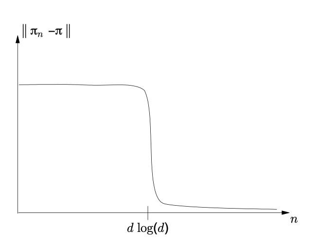
The larger the value of the deck size , the sharper (relative to ) the drop is near .
2.8.3 A random time to exact stationarity
Let’s give a name to each card in the deck (i.e., say the 2 of hearts is card 1, the 3 of hearts is card 2, etc.). Suppose we start with the deck in pristine order (card 1 on top, then card 2, etc.). Though will never become exactly random, it is possible to find a random time at which the deck becomes exactly uniformly distributed, that is, .
Here is an example of such a random time. Suppose that “card i” always refers to the same card (like, say, card 52, the ace of spades), whereas “top card,” “card in position 2,” etc. are just about cards at the time of consideration. Also note that we may describe a sequence of shuffles simply by a sequence of iid random vacriables uniformly distributed on : just say that the -th shuffle moves the top card to position . Define the following random times:
and
It is not hard to see that has the desired property and that is uniformly distributed. To understand this, start with . At time , we know that some card is below card 52; we don’t know which card, but that will not matter. After time we continue to shuffle until , at which time another card goes below card 52. At time , there are 2 cards below card 52. Again, we do not know which cards they are, but conditional on which 2 cards are below card 52, each of the two possible orderings of those 2 cards is equally likely. Similarly, we continue to shuffle until time , at which time there are some 3 cards below card 52, and, whatever those 3 cards are, each of their (3!) possible relative positions in the deck is equally likely. And so on. At time , card 52 has risen all the way up to become the top card, and the other 51 cards are below card 52 (now we do know which cards they are), and those 51 cards are in random positions (i.e. uniform over 51! possibilities). Now all we have to do is shuffle one more time to get card 52 in random position, so that at time , the whole deck is random.
Let us find . By the definitions above, So
Analogously, if the deck had cards rather than 52, we would have obtained (for large ), where is now a random time at which the whole deck of cards becomes uniformly distributed on .
2.8.4 Strong Stationary Times
As we have observed, the random variable that we just constructed has the property that . also has two other important properites. First, is independent of . Second, is a stopping time, that is, for each , one can determine whether or not just by looking at the values of . In particular, to determine whether or not it is not necessary to know any future values .
DEFINITION: A random variable satisfying
- is a stopping time,
- is distributed as , and
- is independent of
is called a strong stationary time.
What’s so good about strong stationary times?
LEMMA: If is a strong stationary time for the Markov chain , then for all .
This tells us that strong stationary times satisfy the same inequality derived for coupling times.
2.8.5 Proof of threshold phenomenon in shuffling
Let denote . The proof that the threshold phenomenon occurs in the top-in-at-random shuffle consists of two parts. Roughly speaking, the first part shows that is close to 0 for slightly larger than , and the second part shows that is close to 1 for slightly smaller than , where in both cases the meaning of “slightly” is “small relative to .”
Part 1 is addressed in the following result:
Note that for each fixed , is small relative to if is large enough. FINISH THIS SECTION
Ch. 3 – MRFs and HMMs
This section looks at aspects of Markov random fields (MRF’s), hidden Markov models (HMM’s), and their applications.
3.1 MRFs on Graphs and HMMs
A stochastic process is a collection of random variables indexed by some subset of the real line . The elements of are often interpreted as times, in which case represents the state at time of the random process under consideration. The term random field refers to a generalization of the notion of a stochastic process: a random field is still a collection of random variables, but now the index set need not be a subset of . For example, could be a subset of the plane . In this section, we’ll consider as the set of nodes of a graph (the set being at most countable). Important aspects of the dependence among the random variables will be determined by the edges of the graph through a generalization of the Markov property.
NOTATION: Given a graph , we say two nodes are neighbors, denoted , if they are joined by an edge of the graph. We do not consider a node to be a neighbor of itself. the set of neighbors of .
DEFINITION: Suppose we are given a graph with nodes and a neighborhood structure . The collection of random variables is a Markov random field on if
for all nodes
More compact notation: for a subset of nodes , let be the vector We will also write for . HMM’s are Markov random fields in which some of the random variables are observable and others are not. We adopt for hidden random variables and for observed random variables.
3.2 Bayesian Framework
What do we get out of these models & how can we use them? One approach is Bayesian: HMM’s fit nicely in the Bayesian framework. is the object of interest; it is unknown. For example, in modeling a noisy image, could be the true image. We consider the unknown to be random, and we assume it has a certain prior distribution. This distribution, our probabilistic model for , is assumed to be a Markov random field. We also postulate a certain probabilistic model for conditional on . This conditional distribution of given reflects our ideas about the noise of blurring or whatever transforms the hidden true image into the image that we observe.
Given our assumed prior distribution of and condiitonal distribution of , Bayes’ formula gives the posterior distribution of . Thus, given an observed value , in principle we get a posterior distribution over all possible true images, so that (again, in principle) we could make a variety of reasonable choices of our estimator of . For example, we could choose the that maximizes . This is called MAP estimation, where MAP stands for “maximum a posteriori”.
3.3 Hammersley - Clifford Theorem
How do we specify a Markov random field? Compared to the case of Markov chains, we might want to specify in terms of a conditional distribution. The following example suggests why this approach goes wrong.
EXAMPLE: Suppose we are designing a Markov random field for images on the 3x3 lattice:
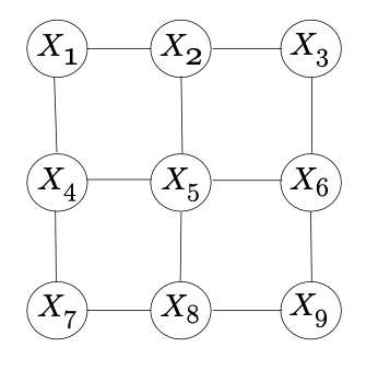
For each pixel, let us specify the conditional distribution of its color given the color of its neighbors. Suppose there are two colors, 0 and 1. But it is possible to specify conditional distributions for each pixel that lead don’t work, i.e., there might be no joint distribution having the given conditional distributions.
In general, we can’t expect to specify a full set of conditional distributions as above. Fortunately, the Hammersley-Clifford Theorem says that a random field’s having the Markov property is equivalent to its having a Gibbs distribution, which is a friendly sort of distribution. Thus, instead of worrying baout specifying our MRF’s in terms of consistent conditional distributions, we can just consider Gibbs distributions, which are simple to write down and work with.
Some definitions needed to state HC:
DEF: A set of nodes is complete if all distinct nodes in are neighbors of each others. A clique is a maximal complete set of nodes.
DEF: Let be a finite graph. A Gibbs distribution with respect fo is a probability mass function that can be expressed in the form
where each is a function that depends only on the values of at the nodes in the clique . That is, the function satisfies if .
By combining functions for sets that are subsets of the same clique, we see that we can further reduce the product in the definiton of Gibbs distribution to
THM (HAMMERSLEY-CLIFFORD): Suppose that has a positive joint probability mass function. is a Markov random field on iff has a Gibbs distribution with respect to .
EXAMPLE: A Markov chain has joint distribution of the form .
By defining and for , we see that this product is a Gibbs distribution on the graph
PROP: Suppose is a Markov random field on the graph with the neighborhood structure . Write , where and are the sets of nodes in corresponding to the and random variables, respectively. Then the marginal distribution of is a Markov random field on , where two nodes are neighbors if either
- They were neighbors in the original graph, or
- There are nodes such that .
The conditional distribution of given is a Markov random field on the graph , where nodes and are neighbors if , that is, if were neighbors in the original graph.
3.4 Long range dependence in the Ising model
For this section, we will work in . For each there is a binary random variable taking values in . The Ising model gives a joint probability distribution for these random variables.
We consider a special case of the Ising model as follows.
For a configuration of +1’s and -1’s at the ndoes of a finite subset of , let denote the number of “odd bonds” in , that is, the number of edges such that . Then, under the Ising model, a configuration has a probability proportional to where is a positive parameter of the distribution (typically <1). The chocie corresponds to the uniform distribution, giving equal probability to all congiruations. Distributions with small strongly dicourage odd bonds, placing large probability on configurations with few odd bonds.
For the case , the model corresponds to a stationary Markov chain with probability transition matrix
Basic Limit Theorem tells us
Thus, the state is asymptotically independent of information at nodes far away from 0.
We will show that the situation in is qualitatively different, in that the effect of states at remote nodes does not disappear in 2 dimensions.
To state the result, some notation:
Imagine a “cube” of side length centered at 0 in , consisting of lattice points whose coordinates all lie between and :
Let denote the boundary points of the cube , that is, the points having at least one coordinate equal to .
Let denote the Ising probability of , conditional on for all . Similarly, let denote probabilities conditional on ’s on the boundary.
THEOREM: For the Ising model on , the effect of the boundary does not disappear. In particular, there exists such that remains below for all , no matter how large.
3.5 Hidden Markov Chains
3.5.1 Model overview
The hidden Markov chain model is a MRF in which some of the random variables are observed and others are not (hence hidden). In the graph structure for the hidden Markov chain, the hidden chain is and the observed process if .
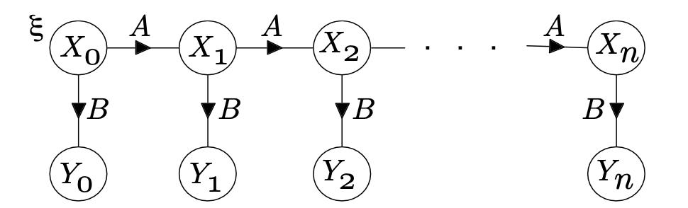
Edges join to both and . The model is parametrized by a marginal distribution of and, if we assume time-homogeneity of the transition matrices, by two transition matrices and , where and
Let us write for the vector of all parameters. If there are states possible for each of the hidden random varirables and oucomes possible for the observed random variables, then is a vector of probabilities, is a probability transition matrix, and is a matrix, each of whose rows is a proabbility mass function.
The hidden Markov chain is pretty general. Examples of cases include
- One hidden state possible for each . Then is just the transition matrix, is , and the process is simply an iid sequence, where each has probability mass function given by . So iid sequences are a special case of the hidden Markov chain model
- If and is the identity matrix, then for all , so Markov chains are a special case of the hidden Markov chain
3.5.2 How to calculate likelihoods
The likelihood function is the probability of the observed data, as a function of the parameters of the model. The tricky aspect is we observe only the ’s, so that
This is a large sum. If the size of the state space of the hidden variables is just , the sum still has terms. Without a way around this computational issue, the hdiden Markov chain model would be of little pratical use. However, it turns out that we can do these calculations in time linear in .
We will denote the state space for the hidden variables by .
We are thinking of the observed values as fixed here–we know them, and will denote them by . For each and for each , define
We can calculate the function immediately:
Note the simple recursion that expressed in terms of :
The sum in the recursion
is fairly modest in comparison. Using the recursion to calculate the function from involves a fixed amount of work, and the task gets no harder as increases. Thus, the amount of work to calculate all of the probabilities for and is linear in .
Having completed the recrusion to calculate the function , the likelihood is simply
The above probabilities are called “forward” probabilities. In a similar manner, we can calculate the “backward” probabilities
by using the recursion
3.5.3 Maximum Likelihood and the EM algorithm
Without an organized method for changing , it is hard to find the that maximizes the likelihood. The EM algorithm is a method for finding maximum likelihood estimates that is applicable to many statistical problems, including hidden Markov chains.
PROP: For and two probability mass functions on we have
A brief description of EM algorithm. We’ll assume are discrete random variables or vectors, so probs are given by sums rathers than integrals.
We want to find the maximizing where . The EM algorithm repeats the following update that is guaranteed to increase the likelihood at each iteration.
Let denote the current value of . Replace by , the value of that maximizes
Why does it work? For a given , define We will see that, in order to have we do not need to find maximizing , but rather it is enough to find a such that
PROP: If then
3.5.4 Applying the EM algorithm to a hidden Markov chain
Consider a hidden Markov chain for , where the r.v.s are observed and the r.v.s are hidden. The model is parametrized by for the distribution of , the prob transition matrix for chain and the prob transition matrix from to .
To describe one iteration of the EM method, imagine our current guess for is We want a new guess that has higher likelihood.
FINISH THIS SECTION PG 107…
In summary, to do EM on hidden Markov chain model:
- Start with some choice of parameter values
- Calculate forward and backward probabilities for and (all with taken as ).
- Calculate the quantities for . These could all be stored in a array.
- Define:
- Replace by and repeat.
3.6 Gibbs Sampler
Terms like “Markov chain Monte Carlo” and “Markov sampling” refer to methods for generating random samples from given distributions by running Markov chains. Although such methods have quite a long history, they have become the subject of renewed interest in the last decade, particularly with the introduction of the “Gibbs sampler” by Geman and Geman (1984), who used the method in a Bayesian approach to image reconstruction. The Gibbs sampler itself has enjoyed a recent surge of intense interest within statistics community, spurred by Gelfand and Smith (1990), who applied the Gibbs sampler to a wide variety of inference problems.
Recall that a distribution being “stationary” for a Markov chain means that, if then for all . The basic phenomenon underlying all Markov sampling methods is the convergence in distribution of a Markov chain to its stationary distribution: If a Markov chain has stationary distribution , then under the conditions of the Basic Limit Theorem, the distribution of for large is close to . Thus, in order to generate an observation from a desired distribution , we find a Markov chain that has as its stationary distribution. The Basic Limit Theorem then suggests that running or simulating the chain until a large time will produce a random variable whose distribution is close to the desired . By taking large enough, in principle we obtain a value that may for practical purposes be considered a random draw from the distribution .
The Gibbs sampler is a way of constructing a Markov chain having a desired stationary distribution. A simple setting that illustrates the idea involves a probability mass function of the form . Suppose we want to generate a random vector . Denote the conditional probability distributions by and . To perform a Gibbs sampler, start with any initial point . Then generate from the conditional distribution , and generate from the conditional distribution . Continue on in this way, generating from the conditional distribution and from the conditional distribution , and so on. Then the distribution is stationary for the Markov chain .
To see this, suppose . In particular, is distributed according to the -marginal of , so that, since is drawn from the conditional distribution of given , we have . Now we use the same reasoning again: is distributed according to the -marginal of , so that . Thus, the Gibbs sampler Markov chain has the property that if then —that is, the distribution is stationary.
Simulating a Markov chain is technically and conceptually simple. We just generate the random variables in the chain, in order, and we are done. However, the index set of a Markov random field has no natural ordering in general. This is what causes iterative methods such as the Gibbs sampler to be necessary.
The Gibbs sampler is well suited to Markov random fields, since it works by repeatedly sampling from the conditional distribution at one node given the values at the remaining nodes, and the Markov property is precisely the statement that these conditional distributions are simple, depending only on the neighbors of the node.
Ch. 4 – Martingales
4.2 Definitions
Notation: Given a process , let denote the portion of the process from time up to time .
DEF: A process is a martingale if
Alternatively, A process is a martingale w.r.t another process if
The crux of the definition is a “fair game” sort of requirement. If we are playing a fair game, we expect neither to win nor to lose money on the average. Given the history of our fortunes up to time , our expected fortune at the future time should just be the fortune that we have at time .
A minor technical condition: we also require for all s.t. the coniditional expectations in the definition are guaranteed to be well-defined.
How about submartingales and supermartingales? These are processes that are “better than fair” and “worse than fair,” respectively.
DEF: A process is a submartingle w.r.t. a process if for each .
{X_n} is a supermartingale w.r.t if for each .
4.3 Examples
See book
4.4 Optional Sampling
Optional sampling property is a “conservation of fairness” type property.
By the “fair game” property, for all . This implies that
That is, one can stop at any predetermined time , like , and their winnings will be fair: .
Fairness is also conserved in many cases, but not in all cases (i.e., if one stops at a time that is not predetermined, but random (depending on the observed sample path of the game)). The issue of optional sampling is this:
If is a random time, that is, is a nonnegative random variable, does the equality still hold?
There are two sorts of things that shouldn’t be allowed if we want fairness to be conserved:
- shouldn’t be able to take an indefinitely long time to stop. for example, a simple symmetric random walk with equal probabilities of going + or - 1. to stop at time then clearly this is not fair.
- shouldn’t be able to “take back” moves. i.e., shouldn’t be able to have information up to time , then go back to some time and claim to stop at .
In fact, ruling out these two sorts of behaviors leaves a class of random times at which the optional sampling statement holds. Disallowing arbitrarily long times is done by assuming bounded. Random times that disallow the gambler from peeking ahead into the future are called stopping times.
DEF: A random variable taking values in the set is a stopping time w.r.t. the process if for each integer , the indicator random variable is a function of .
The main optional sampling result:
THM: Let be a martingale w.r.t. and let be a bounded stopping time. Then .
Now we generalize by
- applying to general supermartingales rather than martingales
- replacing the times and with two stopping times s.t. .
4.5 Stochastic integrals and option pricing in discrete time
oh my great goodness
4.6 Martingale convergence
Intuition: suppose we are playing a supermartingale with initial fortune . Suppose we adopt the strategy of stopping once our fortune exceeds . Our expected reward is at least . But we expect to lose money on a supermartingale, so this expected reward should be no larger than out initial fortune. Then .
4.7 Stochastic approximation
We observe the random variables
where the random variables are subject to our choice and are assumed to be iid “noise” random variables with mean 0 and variance 1. THe function is unknown, and we do not know or observe the noise r.v.s, only the ’s.
Robbins-Monro iteration: a simple way of choosing given the previously observed values.
Some assumptions:
- has a unique but unknown zero
- for
- for
We want to find . Can we have a method of choosing values such that as ?
Suppose we are given a suitable sequence of positive numbers . Then, given , we define according to the recursion
This iteration is qualitatively reasonable. If positive, based on our assumptions about , we would guess that . So we want to be smaller than , which works (if then ), and vice versa.
How should we choose ? We want to converge to something () as , so we need as .
THM: Let and let . Consider the sequence generated by the recursion
where we assume the following conditions:
- the r.v.s are independent, with iid having mean 0 and variance 1.
- for some , we have for all (this incorporates the assumption ).
- for all
- each a nonnegative number and
-
See proof in paper
Ch. 5 – Brownian Motion
Markov processes in discrete time and discrete state space.
Markov processes with continuous sample paths are called diffusions. Brownian motion is the simplest diffusion.
5.1 Definitions
DEF: A standard Brownian motion (SBM) is a stochastic process having
1. continuous paths,
2. stationary, independent increments, and
3. for all .