ISLR

Summary

Skimmed this book out of curiosity & did not finish b/c lack of proofs and overlap, see ESL.

Return to all notes

Ch.1 – Introduction

Notation:

• $P$ the number of variables available for use in making predictions (i.e. $n$ observations and $p$ features)
• $x_{ij}$ the $jth$ variable for the $ith$ observation, where $i = 1, 2, ..., n$ and $j=1,2,...,p$. $X$ a $n \times p$ matrix with $x_{ij}$ as entries
• Matrices are in bold, i.e. A, v.s. random variables as capital normal $A$

Ch.2 – Statistical Learning

Observe a quantiative response $Y$ and $p$ different predictors $X_1, ..., X_p$. We assume there is some relationship b.t. $Y, X = (X_1, ..., X_p)$:

$$Y = f(X) = \epsilon.$$

Statistical learning refers to a set of approaches for estimating $f$.

2.1.1 Why estimate f?

Two main reasons: prediction & inference.

Prediction

In many situations, a set of inputs $X$ are readily available, but the output $Y$ cannoot be easily obtained. In this setting, since the error term averages to zero, we can predict $Y$ using

$$\hat Y = \hat f (X),$$

where $\hat f$ represents our estimate for $f$, and $\hat Y$ represents the resulting prediction for $Y$. $\hat f$ is often treated as a black box.

The accuracy of $\hat Y$ as a prediction for $Y$ depends on the reducible and irreducible error. In general, $\hat f$ will not be a perfect estimate for $f$; this error is reducible because we can potentially improve the accuracy. However, $Y$ itself is also a function of $\epsilon,$ which cannot, by definition, be predicted by $X$. This is the irreducible error.

Consider a given estimate $\hat f$ and a set of predictors $X$, which yields the prediction $\hat Y = \hat f(X)$. Assume for now that both $\hat f, X$ are fixed. Then,

$$\begin{align*} E(Y - \hat Y)^2 &= E[f(X) + \epsilon - \hat f(X)]^2 \\ &= [f(X) - \hat f(X)]^2 + \text{Var}(\epsilon), \end{align*}$$

where the first term is reducible and the second term is irreducible. $E(Y - \hat Y)^2$ the EV of the squared difference between predicted and actual value of $Y$. $\Var(\epsilon)$ the variance associated with the error term $\eps$.

Inference

We are often interested in understanding how $Y$ is affected as $X_1, ..., X_p$ change. We wish to estimate $f$, but are not necessarily going to make predictions for $Y$. Now $f$ cannot be treated as a black box, because we need to know its exact form. We might be interesting in asking,

• Which predictors are associated with the response?
• What is the relationship between the response and each predictor?
• Can the relationship between Y and each predictor be adequately summarized using a linear equation, or is the relationship more complicated?

2.1.2 How do we estimate f?

Explore linear and nonlinear approaches to estimating $f$. These methods generally share certain characteristics. Overview of these shared char’s in this section/

Will assume we have observed $n$ diff data points (training data). $x_{ij}$ the value of the $j$-th predictor for observation $i$, where we have $n$ observations and $p$ features. $y_i$ the response variable for the $i$-th observation.

We want to find $\hat f$ such that $Y \approx \hat f (X)$ for any observation $(X, Y)$.

Parametric Methods

Parametric methods involve a 2-step model-based approach.

• Make an assumption about the functional form of $f$. Ex: $f$ is linear in $X$, $f(X) = \beta_0 + \beta_1 X_1 + ... + \beta_p X_p.$ This is a linear model. Once we have assumed $f$ is linear, the problem of estimating $f$ is simplified. We need only estimate the $p+1$ coefficients.

• After a model has been selected, we need a procedure that uses the training data to fit or train the model. In the case of the linear model, the most common approach is referred to as ordinary least squares, but there are many ways.

“Parametric” = we fix the number of parameters that need to be estimated. Simplifies the estimation but potentially may be poor estimate if we choose a model too far from true $f$. In general, fitting a more flexible model requires estimating a greater number of parameters, but this can lead to overfitting, where models follow the errors (noise) too closely.

Non-parametric Methods

Do not make explicit assumptions abt the functional form of $f$. Seek an estimate of $f$ that gets as close to data points as possible without being too “rough or wiggly.” Such approaches are advantageous because they have the potential to accurately fit a wider range of possible shapes for $f$, but a very large number of observations is required for an accurate estimate.

2.1.3 Trade-off bt. Prediction Accuracy and Model Interpretability

One might ask: why would we ever choose to use a more restrictive method instead of a very flexible approach? There are several reasons we might prefer a more restrictive model. If we are mainly interested in inference, then restrictive models are much more interpretable. In some settings, however, we are only interested in prediction, and teh interpretability of the predictive model is simply not of interest.

2.1.4 Supervised vs. Unsupervised Learning

Most statistical learning problems fall into one of two categories: supervised or unsupervised. Supervised learning means for each observation of the predictor measurements, there is an associated response measurement. Unsupervised learning is when for every observation $i= 1, ..., n$ we observe a vector of measurements $x_i$ but no associated response $y_i$. What sort of statistical analysis is then possible?

We can seek to understand the relationships between the variables or between the observations. One stat learning tool we might use is cluster analysis, or clustering. The goal is to ascertain, on the basis of $x_1, ..., x_n$, whether the observations fall into relatively distinct groups.

Semi-supervised learning occurs when we have predictor and response measurements for $m < n$ observations, and the remaining $n-m$ observations have no response measurement.

2.1.5 Regression vs. Classification

Variables can be quantitative or qualitative (categorical). Quantitative variables take on numerical values. We tend to refer to problems with a quantitative response as regression problems, and qualitative responses as classification problems.

2.2 Assessing Model Accuracy

2.2.1 Measuring Quality of Fit

In order to evaluate the performance of a stat learning method on a given data set, we need some way to measure how well its predictions match the observed data.

In the regression setting, the most commonly used measure is the mean squared error (MSE)

$$MSE = \frac{1}{n} \sum_{i=1}^n (y_i - \hat f (x_i))^2,$$

where $\hat f(x_i)$ is the prediction $\hat f$ gives for the $i$-th observation. The MSE will be small if the pred responses are very close to the true responses, and will be large if for some of the observations, the pred and true responses differ substantially.

The MSE above is computed using the training data and should be referred to as the training MSE. In general, we are interested in the accuracy of the predictions that we obtain when we apply our method to previously unseen test data. We would like to select a method that minimizes the test MSE.

In some settings, we may have a test data set available. If no test observations are available, one cannot just choose the approach minimizing the training MSE.

As the flexibility of the statistical learning method increases, we observe a monotone decrease in the training MSE and a U-shape in the test MSE. This is a fundamental property of statistical learning that holds regardless of the method and data set. When a given method yields a small training MSE but a large test MSE, we are said to be overfitting.

Throughout this book, we discuss a variety of approaches that can be used in practice to estimate the proper minimum test MSE.

2.2.2 The Bias-Variance Trade-Off

The U-shape observed in the test MSE curves turns out to be the result of two competing statistical learning methods. The expected test MSE, for a given $x_0$, can always be decomposed into the sum of three fundamental quantities: the variance of $\hat f(x_0)$, the squared bias of $\hat f(x_0)$, and the variance of the error terms $\eps$:

$$\E \left( y_0 - \hat f(x_0) \right)^2 = \Var(\hat f(x_0)) + [\text{Bias}(\hat f (x_0))]^2 + \Var(\eps).$$

Here $\E \left( y_0 - \hat f(x_0) \right)$ defines the expected test MSE, the average test MSE we would obtain if we estimated $f$ using a large number of training sets, and tested at each $x_0$. The overall expected test MSE can be computed by averaging $\E \left( y_0 - \hat f(x_0) \right)$ over all possible values of $x_0$ in the test set.

In order to minimize the expected test error, we need to select a method that achieves both low variance and low bias.

Variance refers to the amount by which $\hat f$ would change if we estimated it using a different training data set. In general, more flexible statistical methods have higher variance.

Bias introduced by approximating a real-life problem by a much simpler model. For example, linear regression assumes a linear relationship, which is unlikely in real life, resulting in bias in the estimation of $f$. Generally, more flexible methods result in less bias.

As a general rule, as we use more flexible methods, the variance will increase and the bias will decrease. The relative rate of change of these two quantities determines whether the test MSE increases or decreases. The relationship between bias, variance, and test set MSE is referred to as the bias-variance trade-off. The challenge lies in finding a method for which both the variance and squared bias are low.

In a real life situation in which $f$ is unobserved, it is generally not possible to explicitly compute the test MSE, bias, or variance for a stat learning method.

2.2.3 The Classification Setting

Suppose we seek to estimate $f$ on the basis of $\{(x_1, y_1, ..., (x_n, y_n)\}$ where $y_1, ..., y_n$ are qualitative. The most common approach for quantifying the accuracy is the training error rate, the proportion of mistakes that are made if we apply our estimate $\hat f$ to the training observations:

$$\frac{1}{n} \sum_{i=1}^n I(y_i \neq \hat y_i).$$

The test error rate associated with a set of test observations of the form $(x_0, y_0)$ is given by

$$\text{Ave}(I(y_0 \neq \hat y_0)),$$

where $\hat y_0$ is the predicted class label that results from applying the classifier to the test observation with predictor $x_0.$

The Bayes Classifier

It is possible to show that the test error rate is minimized, on average, by a very simple classifier that assigns each observation to the most likely class, given its predictor values. In other words, we should simply assign a test observation with a prediciton vector $x_0$ to the class $j$ for which

$$\P(Y = j | X = x_0)$$

is largest. This simple classifier is called the Bayes classifier.

The Bayes classifier’s prediction is determined by the Bayes decision boundary.

The Bayes classifier produces the lowest possible test error rate, called the Bayes error rate. Since the Bayes classifier will always choose the class for which $\P(Y = j | X = x_0)$ is largest, the error rate at $X= x_0$ will be $1- \text{max}_j \P(Y = j | X =x_0).$ In general, the overall Bayes error rate is given by

$$1 - \E \left(\text{max}_j \P (Y=j | X)\right),$$

where the expectation averages the probability over all possible values of $X$.

K-Nearest Neighbors

In theory, we would like to predict qualitative responses using the Bayes classifier. But for real data, we don’t know the cond. distribution of $Y$ given $X$, so computing the Bayes classifier is impossible. The Bayes classifier serves as an unattainable gold standard against which to compare other models. Many approaches try to estimate the cond. dist. of $Y$ given $X$, then classify a given observation to the class with the highest estimated probability. One such example is the K-nearest neighbors (KNN) classifier.

Given a positive integer $K$ and a test observation $x_0$, the KNN classifier first identifies the $K$ points in the training data that are closest to $x_0$, represented by $N_0$.

It then estimates the conditional probability for class $j$ as the fraction of points in $N_0$ whose response values equal $j$:

$$\P (Y=j | X=x_0) = \frac{1}{K} \sum_{i \in N_0} I(y_i = j).$$

Finally, KNN applies Bayes rule and classifies the test observation $x_0$ to the class with the largest probability.

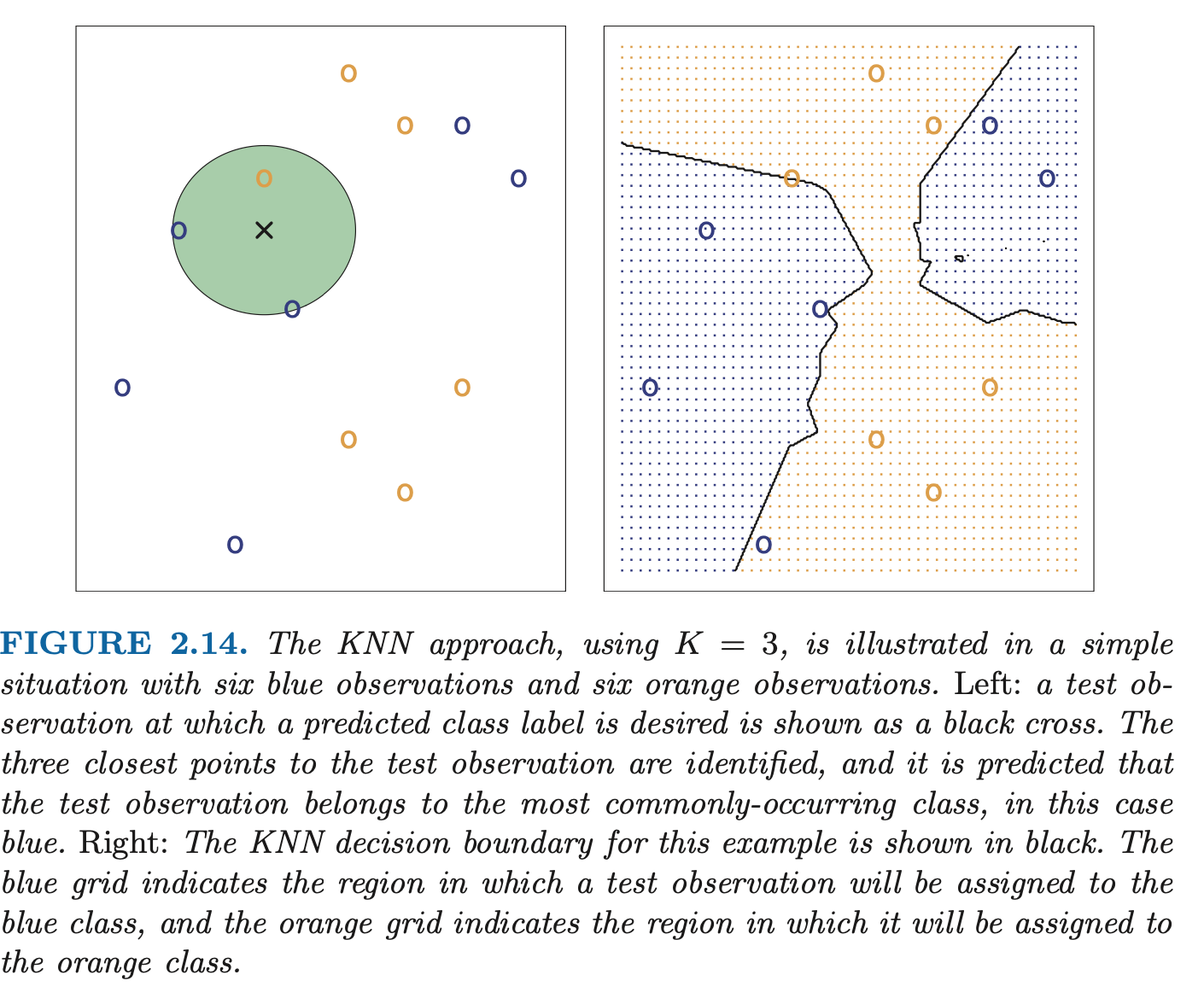
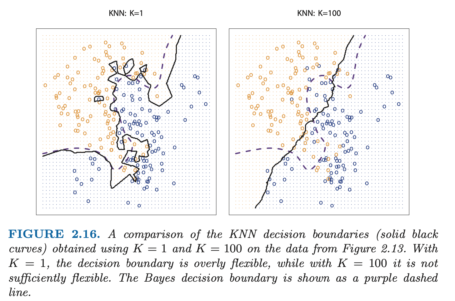
The choice of $K$ has a drastic effect on the KNN classifier obtained. As $K$ grows, the method becomes less flexible and produces a decision boundary that is close to linear (low-variance, high-bias).

Ch. 3 – Linear Regression

3.1 Simple Linear Regression

Simple linear regression assumes there is an approximately linear relationship between $X$ and $Y$.

$$Y \approx \beta_0 + \beta_1 X.$$

Sometimes described as “regressing $Y$ on $X$” or “$Y$ onto $X$”. Once we have used our training data to produce estimates $\hat \beta_0, \hat \beta_1$ for the model coefficients, we can predict

$$\hat y = \hat \beta_0 + \hat \beta_1 x.$$

3.1.1 Estimating the Coefficients

In practice, the parameters are unknown. We must use data to estimate the coefficients. Suppose we have $n$ observation pairs. We’ll use least squares, the most common approach to determining closeness.

Let $\hat y_i = \hat \beta_0 + \hat \beta_1 x_i$ be the prediction for $Y$ based on the $i$-th value of $X$. Then $e_i = y_i - \hat y_i$ represents the $i$-th residual.

We define the residual sum of squares (RSS) as

$$\text{RSS} = e_1^2 + e_2^2 + ... + e_n^2,$$

or equivalently as

$$\text{RSS} = (y_1 - \hat \beta_0 - \hat \beta_1 x_1)^2 + (y_2 - \hat \beta_0 - \hat \beta_1x_2)^2 + ...+(y_n - \hat \beta_n - \hat \beta_1 x_n)^2.$$

The least squares approach choose $\hat \beta_0$ and $\hat \beta_1$ to minimize the RSS. Using calculus, one can show that the minimizers are

$$\begin{align*} \hat \beta_1 &= \frac{ \sum_{i=1}^n (x_i - \bar x)(y_i - \bar y)}{\sum_{i=1}^n (x_i - \bar x)^2}, \\ \hat \beta_0 &= \bar y - \hat \beta_1 \bar x, \\ (3.4) \end{align*}$$

where $\bar y = \frac{1}{n} \sum_{i=1}^n y_i$ and $\bar x = \frac{1}{n}\sum_{i=1}^n x_i$ are the sample means. In other words, the above defines the least squares coefficient estimates for simple linear regression.

3.1.2 Assessing the Accuracy of the Coefficient Estimates

We assume the true relationship between $X,Y$ as $Y =f(X) + \eps$. If $f$ is to be approx as a linear fn, we can write this as

$$Y = \beta_0 + \beta_1X+\eps. (3.5)$$

The model given by this equation (3.5) defines the population regression line: the best linear approximation to the true relationship between $X$ and $Y$. The least squares regression coefficient estimates characterize the least squares line. The true relationship is generally not known for real data, but the least squares line can always be computed using the (3.4) estimates. (think: population mean $\mu$ vs sample mean $\hat \mu$).

If we use the sample mean $\hat \mu$ to estimate $\mu$, this estimate is unbiased: on average, expected $\hat mu$ to equal $\mu$.

Hence, an unbiased estimator does not systematically over- or under-estimate the true parameter.

Next, (again with the pop vs sample mean), recall how we check accuracy of sample mean $\hat \mu$ as an estimate of $\mu$. How far off will a single estimate $\hat \mu$ be off of $\mu$? Generally, we answer this with the standard error of $\hat \mu$, written $\text{SE}(\hat \mu)$.

$$\Var (\hat \mu) = \text{SE}(\hat \mu)^2 = \frac{\sigma^2}{n},$$

for $\sigma$ the standard deviation of each of the realizations $y_i$ of Y. Roughly speaking, the standard error tells us the avg amt that the estimate $\hat \mu$ differs from the actual value $\mu$. It also tells us how this deviation shrinks with $n$.

Similarly, how do we check how close $\hat \beta_0, \hat \beta_1$ are to the true values $\b_0, \b_1$? To compute the standard errors associated with $\hat \b_0$ and $\hat \b_1$, we use the following formulas:

$$\se(\hat \b_0)^2 = \sigma^2 \left[ \frac{1}{n} + \frac{\bar x^2}{\sum_{i=1}^{n}(x_i - \bar x)^2} \right], \se(\hat \b_1)^2 = \frac{\sigma^2}{\sum_{i=1}{n}(x_i - \bar x)^2},$$

where $\sigma^2 = \Var(\eps)$. For these formulas to be strictly valid, we need to assume the errors for reach observation are uncorrelated with common variance $\sigma^2$. In general, $\sigma^2$ is not known, but can be estimated from the data. This estimate is the residual standard error, given

$$\text{RSE} = \sqrt{\text{RSS}/ (n-2)}.$$

Standard errors can be used to compute confidence intervals. A 95% confidence interval is defined as a range of values such that with 95% probability, the r ange will contain the true unknown of the parameter. The range is defined in terms of lower and upper limits computed from the sample of data.

For lin reg, 95% confidence interval for $\b_1$ approx $\hat \b_1 \pm 2 \cdot \se(\hat\b_1)$ and similarly for $\b_0$.

Standard errors can also be used to perform hypothesis tests on the coefficients. The most common hypothesis test involves testing the null hypothesis of

$$H_0 : \text{ There is no relationship between } X \text{ and } Y$$

vs the alternative hypothesis

$$H_a: \text{ There is some relationship between } X \text{ and } Y.$$

Mathematically, this corresponds to testing

$$H_0: \beta_1 = 0 \text{ vs. } H_a: \b_1 \neq 0.$$

To test the null hypothesis we need to determine whether our estimate is sufficiently far from zero to be confident that $\beta_1$ is non-zero. How far depends on the accuracy of our estimate. in practice, we compute a t-statistic:

$$t = \frac{\hat \b_1 - 0}{\text{SE}(\hat \b_1)}, (3.14)$$

which measures the number of standard deviations that $\hat \b_1$ is away from 0. If there is no relationship between $X$ and $Y$, we expect (3.14) to have a t-distribution with $n-2$ degrees of freedom. The t-dist has bell shape and for $n >$ about 30, is very similar to the normal dist. So it is easy to compute the prob of observing any value equal to $|t|$ or larger, assuming $\b_1 = 0$. We call this probability the p-value.

Roughly speaking, a small p-value indicates it is unlikely to observe a substantial association between the predictor and the response due to chance, in the absence of any real ssociation between the predictor and the response. Hence, if there is a small p-value, we can infer there is an association b.t. the predictor and response. We reject the null hypothesis, i.e., declare a relationship to exist b.t. $X,Y$. Typical p-value cutoffs for rejecting the null hypothesis are 5% or 1%.

3.1.3 Assessing the Accuracy of the Model

After rejecting the null hypothesis we want to know the extent to which the model fits the data. The quality of a linear regression fit is typically assessed using two related quantities: the residual standard error (RSE) and the $R^2$ statistic.

Recall that associated with each observation is an error term. The RSE is an estimate of the standard deviation of $\eps$ (the avg amt that the response will deviate from the true regression line):

$$\text{RSE} = \sqrt{\frac{1}{n-2}\text{RSS}} = \sqrt{\frac{1}{n-2}\sum_{i=1}^n (y_i - \hat y_i)^2}.$$

The RSE measures a lack of fit. The $R^2$ statistic provides an alternative measure of fit. It is the proportion of variance explained, so it is always between 0 and 1.

$$R^2 = \frac{\text{TSS} - \text{RSS}}{\text{TSS}} = 1 - \frac{\rss}{\tss},$$

where $\tss = \sum (y_i - \bar y)^2$ is the total sum of squares. TSS measures the total variance in the response $Y$, and can be thought of the amount of variability inherent in the response before the regression is performed. RSS measures the amount of variability left unexplained after performing the regression. So $R^2$ is the proportion of variability in $Y$ that can be explained using $X$.

3.2 Multiple Linear Regression

Fitting a separate simple linear reg model for each predictor is not satisfactory (for example, it’s unclear how to make 1 prediction with several different regression equations).

A better approach is to extend to multilinear regression, where each predictor gets a separate slope coefficient in a single model. Suppose we have $p$ distinct predictors. Then the multilinear regression model takes the form

$$Y = \b_0 + \b_1 X_1 + \b_2 X_2 + ... + \b_p X_p + \eps.$$

We interpret $\b_j$ as the average effect on $Y$ of a one unit increase in $X_j$, holding all other predictors fixed.

3.2.1 Estimating the Regression Coefficients

As in simple linear reg, we want to make predictions using the formula

$$\hat y = \hat b_0 + \hat \b_1 x_1 + ... + \hat \b_p x_p.$$

The parameters are again estimated using the same least squares approach, choosing our regression coefficients estimates as those that minimize the sum of squared residuals

$$\begin{align*} \rss &= \sum_{i=1}^n (y_i - \hat y_i)^2 \\ &= \sum_{i=1}^n (y_i - \hat \b_0 - \hat \b_1 x_{i1} - \hat \b_2 x_{i2} - ... - \hat \b_p x{ip}). \end{align*}$$

The muliple regression coefficient estimates are more complex than the simple linear reg coeffs, better represented in matrix form.

3.2.2 Some important questions

• Is at least one of the predictors useful in predicting the response?

  • test null vs. alternative hypothesis (all are 0 vs at least one is non-zero). computed with the F-statistic:

  $$F = \frac{(\tss - \rss) / p}{\rss / (n-p-1)}.$$

  • if the linear model assumptions are correct, the ev of the denom is $\sigma^2$. if the null hypothesis holds, the num is $\sigma^2$. so the null hypothesis should have the F-stat close to 1.
  • if the alternative hypothesis is true, the ev of the numerator $> \sigma^2$, so we expect F-stat greater than 1.
  • again, what determines the F-stat being large enough depends on $n$ and $p$, we can compute the p-value to decide.
  • sps we want to test a subset that $q$ of the coeffs are zero. then we fit a second model using all the variables except for the $q$ coeffs, and sps the rss for that model is $\rss_0$. then the appropriate F-stat is

  $$F = \frac{(\rss_0 - \rss)/q}{\rss/(n-p-1)}.$$

  • if $p>n$ we cannot fit using least squares, so the F-stat cannot be used.

• Do all the predictors help to explain $Y$, or only a subset?

  • the task of determining which predictors are associated with the response is variable selection
  • there are 3 classical approaches to choosing a smaller set of models
    • forward selection: begin with the null model (intercept, 0 predictor), then fit $p$ simple linear regressions and add to the null model the variable resulting in the lowest RSS. then repeat until some stopping rule
    • backward selection: start with all variables, and remove the variable with the largest p value. fit the new (p-1) variable model. repeat until stopping rule
    • mixed selection: start with no variables, and add one by one as in forward. if at any point the p-value for one of the variable rises above a certain threshold, remove that variable. go until all variables have sufficiently low p-value, and all outside variables would have large p-value if added.
  • backward selection cannot be used if $p > n$, while forward selection can always be used. forward selection is a greedy approach and might include variables early on that later become redundant. mixed selection can remedy this.

• How well does the model fit the data?

  • two of the most common measures are the RSE and $R^2$.
    • in multiple linear regression, $Y^2 = \text{Cor}(Y, \hat Y)^2$ (square of correlation between response and fitted linear model)
  • plotting the data can be helpful

• Given a set of predictor values, what response value should we predict, and how accurate is our prediction?

  • three sorts of uncertainty: we are only using estimates of the true population regression coefficients
  • model bias because $f$ may not even be linear
  • irreducible error from the random error in the model

3.3 Other Considerations in the Regression Model

• some predictors may be qualitative (called a factor), for binary (two levels) we introduce a dummy variable 0 or 1
  • for n levels, we add n-1 dummies (the nth is implied if all the n-1 are 0), level with no dummy variable is the baseline

3.3.2 Extensions of the Linear Model

Two important assumptions of the linear regression model that are violated in practice are the additive assumption and linear assumption.

Additive: the effect of changes in a predictor $X_j$ on the response $Y$ is independent of the values of the other predictors.

• removing the additive assumption: including an extra predictor, called an interaction term.
  • hierarchical principle: if we include an interaction in a model, we should also include the main effects, even if the p-values associated with their coefficients are not significant (if the interaction bt $X_1, X_2$ is included, we should include $X_1, X_2$ themselves, even if their own coeff estimates have large p-values)

Linear: the change in the response $Y$ due to a 1-unit change in $X_j$ is constant, regardless of the value of $X_j$.

• a simple way to directly extend linear reg to accommodate non-linear relationships is polynomial regression
  • sps we think that our model with 2 features should include a quadratic term (for $X_2$ being, say, horsepower). then our model is still a multilinear model with $X_1$ and $X_2 = \text{horsepower}^2.$

3.3.3 Potential Problems

When we fit a linear regression model, common problems that may occur are:

• Nonlinearity of the response-predictor relationships

  • plotting residuals against the predictor $x_i$ for simple linear regression, or residuals vs predicted values $\hat y_i$ for multi. ideally, the residual plot will show no discernible pattern

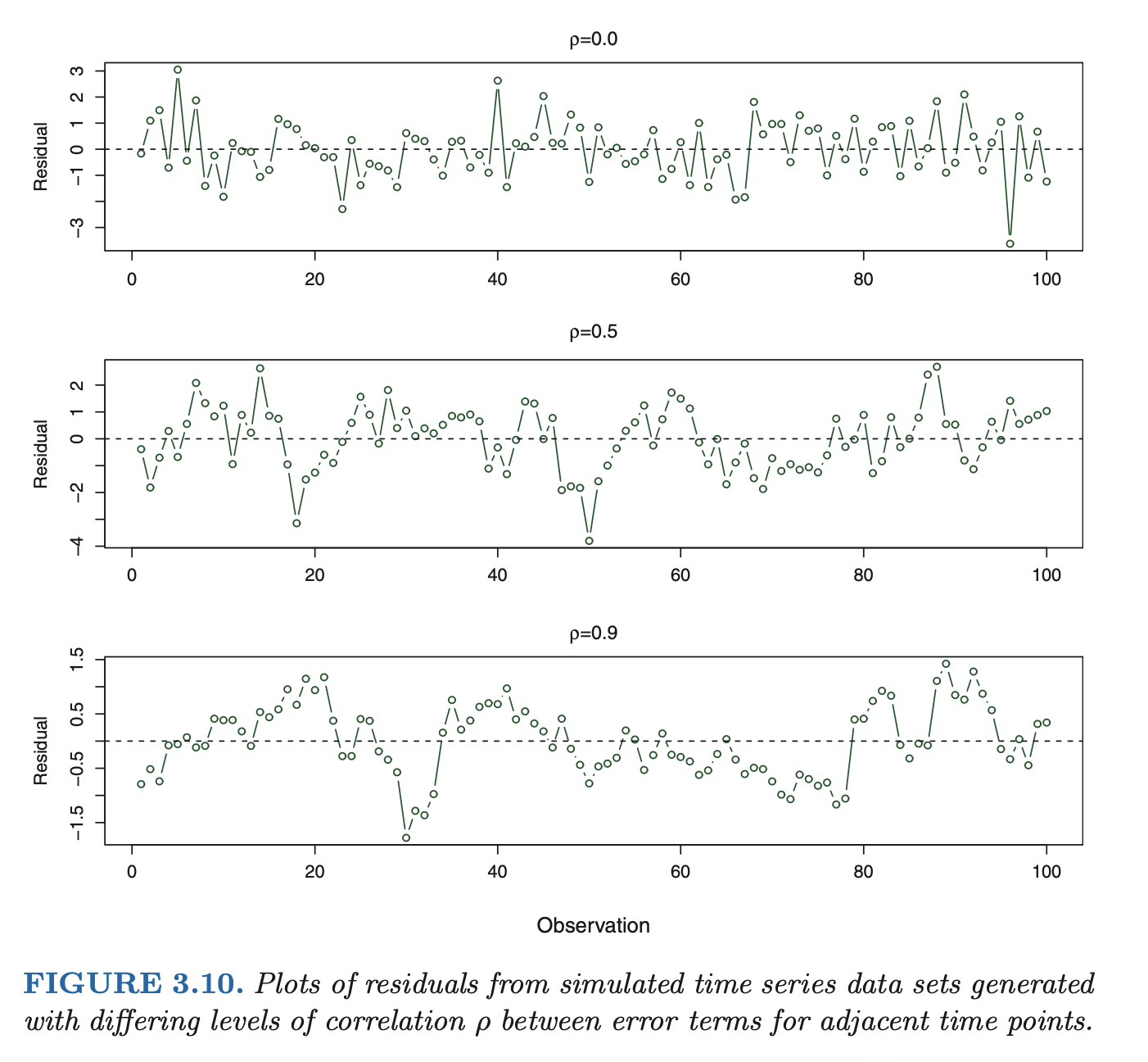
• Correlation of error terms

  • if in fact there is correlation among the error terms, then the estimated standard errors will tend to underestimate the true standard errors. As a result, confi- dence and prediction intervals will be narrower than they should be.
  • in addition, p-values associated with the model will be lower than they should be; this could cause us to erroneously conclude that a parameter is statistically significant. in short, if the error terms are correlated, we may have an unwarranted sense of confidence in our model. as an extreme example, suppose we accidentally doubled our data, leading to observations and error terms identical in pairs. If we ignored this, our standard error calculations would be as if we had a sample of size $2n$, when in fact we have only $n$ samples. Our estimated parameters would be the same for the $2n$ samples as for the $n$ samples, but the confidence intervals would be narrower by a factor of $\sqrt{2}$!

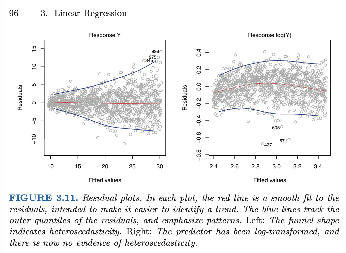
• Non-constant variance of error terms (heteroscedasticity)

  • can be identified from a funnel shape in the residual plot.
  • common situation is when variance of error increases with the value of the response
    • one solution is to transform the response with a concave function (eg log), resulting in a greater amount of shrinkage of larger response
  • sometimes we have a good idea of the variance of each response. if each of the raw observations is uncorrelated, we can fit our model with weighted least squares

• Outliers

  • how large does a point have to be to be an outlier? we can plot the studentized residuals. observations whose studentized residuals are greater than 3 in absolute value are possible outliers

• High-leverage points

  • outliers are when repsonse is unusual, whereas high-leverage is unusual value for $x_i$. we can quantify an observation’s leverage with the leverage statistic. for a simple linear regression,

  $$h_i = \frac{1}{n} + \frac{(x_i - \bar x)^2}{\sum_{i'=1}^n (x_{i'} - \bar x)^2}.$$

  • there is no simple extension to multiple predictors
  • the leverage statistic is always between $1/n$ and $1$, with average $(p+1)/n$. a leverage statistic greatly exceeding that average might mean the corresponding point has high leverage.

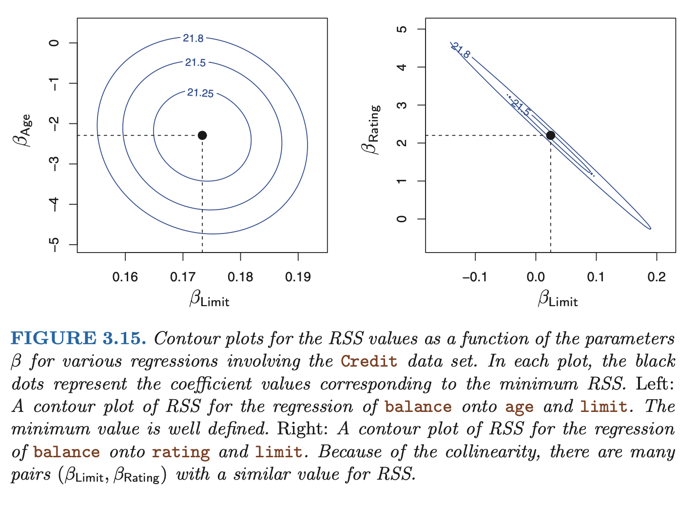
• Collinearity

  • the situation when two or more predictor variables are closely related to one another
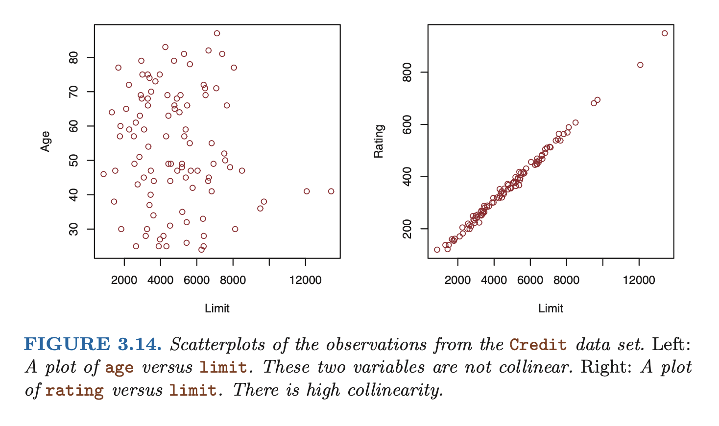
  • collinearity reduces the accuracy of the estimates of the regression coefficients, therefore causing the standard erorr for $\hat \b_j$ to grow. this results in a decline in the t-statistic. then, in the presence of collinearity, we may fail to reject $H_0: \b_j = 0$.
  • a simple way to detect collinearity is to look at the correlation matrix of the predictors. An element of this matrix that is large in absolute value indicates a pair of highly correlated variables, and therefore a collinearity problem in the data. Unfortunately, not all collinearity problems can be detected by inspection of the correlation matrix: it is possible for collinearity to exist between three or more variables even if no pair of variables has a particularly high correlation. this is called multicollinearity
  • a better way to assess multicollinearity is to compute the variance inflation factor (VIF).

  $$\text{VIF}(\hat \b_j) = \frac{1}{1-R^2_{X_j | X_{-j}}},$$

  • where $R^2_{X_j | X_{-j}}$ is the $R^2$ from a regression of $X_j$ onto all of the other predictors. if it is close to 1, then collinearity is present, so the VIF will be large.
  • min VIF is 1 (no collinearity), generally a VIF over 5 or 10 is problematic

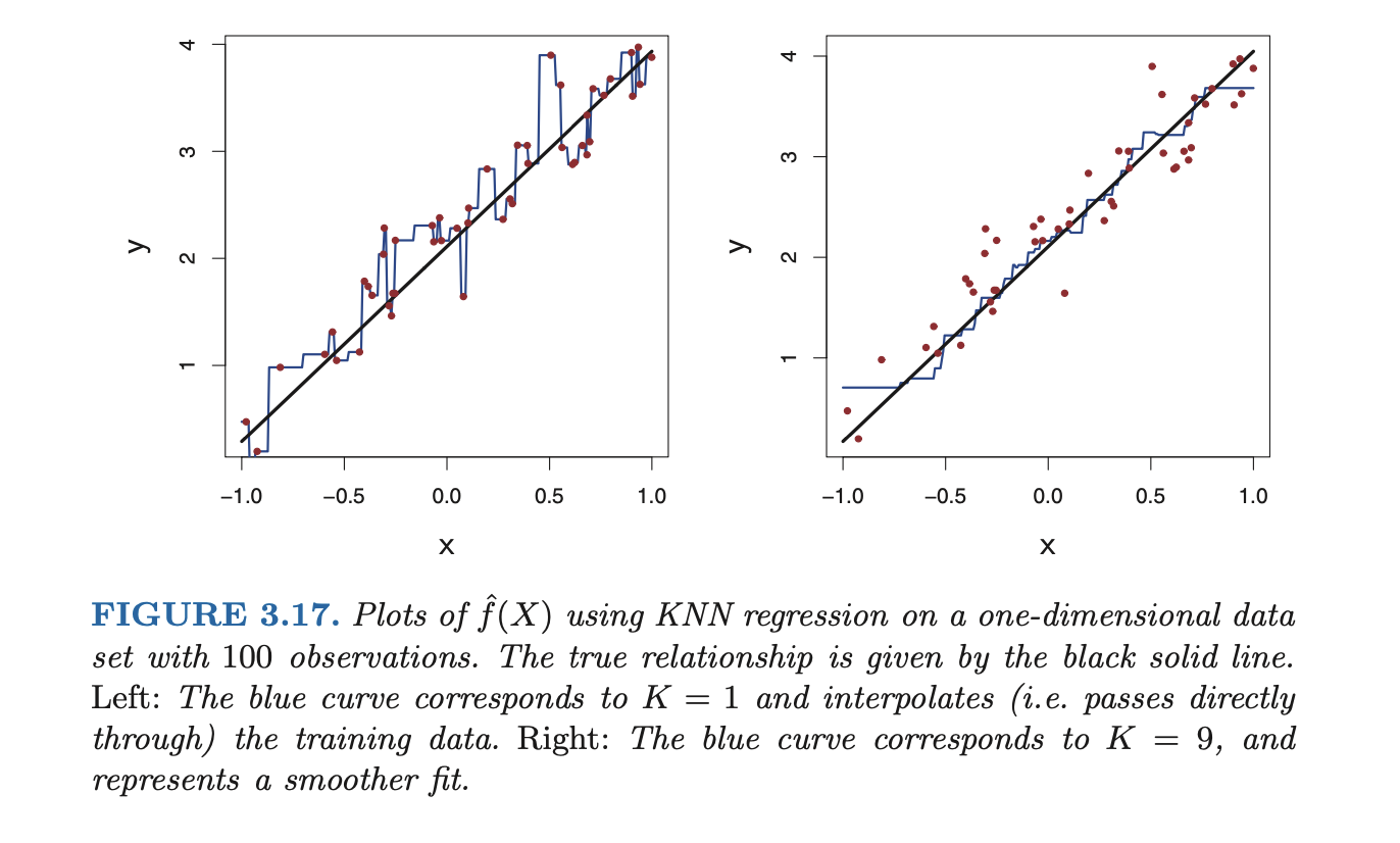
3.5 Comparison of Linear Regression w/ KNN

One of the simplest non-parametric methods is K-nearest neighbors regression (KNN regression).

KNN regression is closely related to the KNN classifier. Given a value $K$ and a prediction point $x_0$, KNN regression first identifies the $K$ training observations closest to $x_0$, represented by $N_0$. It then estimates $f(x_0)$ using the vareage of all the training respponses in $N_0$:

$$\hat f(x_0) = \frac{1}{K} \sum_{x_i \in N_0} y_i.$$

In what setting will a parametric approach such as least squares linear regression outperform a non-parametric approach such as KNN regression? The answer is simple: the parametric approach will outperform the nonparametric approach if the parametric form that has been selected is close to the true form of $f$.

Ch 4 – Classification

• discusses log reg, linear discriminant analysis, and KNN
• in log reg, we use the logistic function and fit the model with maximum likelihood
  • maximum likelihood = finding coefficients to maximimize a likelihood function
• alternative approach to directly modeling two response classes with logistic regression, linear discriminant analysis models the distribution of the predictors separately in each of the response classes, and then use Bayes’ to fliip these into estimates for prob of each class given X.
• both logistic re- gression and LDA produce linear decision boundaries
  • Since logistic regression and LDA differ only in their fitting procedures, one might expect the two approaches to give similar results. This is often, but not always, the case. LDA assumes that the observations are drawn from a Gaussian distribution with a common covariance matrix in each class, and so can provide some improvements over logistic regression when this assumption approximately holds. Conversely, logistic regression can outperform LDA if these Gaussian assumptions are not met.
• KNN is a completely non-parametric approach: no assumptions are made about the shape of the decision boundary. There- fore, we can expect this approach to dominate LDA and logistic regression when the decision boundary is highly non-linear. On the other hand, KNN does not tell us which predictors are important
• Finally, QDA serves as a compromise between the non-parametric KNN method and the linear LDA and logistic regression approaches. Since QDA assumes a quadratic decision boundary, it can accurately model a wider range of problems than can the linear methods. Though not as flexible as KNN, QDA can perform better in the presence of a limited number of training observations because it does make some assumptions about the form of the decision boundary.

Ch 5 – Resampling Methods

• resampling methods are when you repeatedly draw samples from a training set and refit a model of interest on each sample to obtain additional information about the fitted model
• can be computationally expensive
• two most commonly used methods are cross validation and the bootstrap
• evaluating a model’s performance = model assessment
• selecting the proper level of flexibility for a model = model selection

5.1 Cross Validation

• training error can differ from test error by a lot
• a class of methods that estimate the test error by holding out a subset of the training observations from the fitting process

5.1.1 Validation Set Approach

• randomly divide available observations into training set and validation set
• two drawbacks:
  • validation estimate of test error rate can be highly variable
  • only a subset of the observations are used in training, so validation set error rate may tend to overestimate test error rate

5.1.2 Leave One Out Cross Validation

• LOOCV is when we only use a single observation for the validation set, and the remianing observations are used for training
• now the estimate for test error is approximately unbiased, but highly variable. so we repeat the procedure by doing LOOCV by holding out the next observation, and so on.
• LOOCV estimate for test MSE is the average of the $n$ test error estimates:

$$\text{CV}_n = \frac{1}{n} \sum_{i=1}^n \text{MSE}_i.$$

Advantages over validation set approach:

• less bias, so tends not to overestimate the test error as much
• validation approach yields diff results when applied repeatedly due to randomness in training / val set splits. performing LOOCV multiple times always yields the same results

Note: LOOCV has the potential to be expensive to implement: we have to fit the model $n$ times. time consuming if $n$ large. However, with least squares linear or polynomial regression, the cost of LOOCV is the same as that of a single model fit, because the following formula holds:

$$\text{CV}_n = \frac{1}{n} \sum_{i=1}^n (\frac{y_i - \hat y_i}{1-h_i})^2,$$

where $\hat y_i$ is the $i$-th fitted value from the original least squares fit, and $h_i$ is the leverage.

5.1.3 k-Fold Cross Validation

• randomly divide the observations into $k$ folds of approx. equal size
• first fold is val, and method is refit on the remaining $k-1$ folds. calculate MSE for each time and repeat procedure $k$ times. the $k$-fold CV estimate is the average:

$$\text{CV}_k = \frac{1}{k}\sum_{i=1}^k \text{MSE}_i.$$

Clearly, LOOCV is a special case of $k$-fold CV where $k=n$. In practice, one typically does $k$ fold CV with $k=5$ or $k=10$.

Computational advantage over LOOCV.

5.1.4 Bias-Variance Trade-Off for k-Fold CV

$k$-fold CV also often gives more accurate estimates of the test error rate than LOOCV, which has to do with a bias-variance trade-off.

Obviously, in terms of bias reduction, LOOCV is preferable to $k$-fold CV. But LOOCV has higher variance than $k$-fold CV with $k < n$:

• When we perform LOOCV, we are in effect averaging the outputs of n fitted models, each of which is trained on an almost identical set of observations; therefore, these outputs are highly (positively) correlated with each other. In contrast, when we perform $k$-fold CV with $k < n$, we are averaging the outputs of k fitted models that are somewhat less correlated with each other, since the overlap between the training sets in each model is smaller. Since the mean of many highly correlated quantities has higher variance than does the mean of many quantities that are not as highly correlated, the test error estimate resulting from LOOCV tends to have higher variance than does the test error estimate resulting from $k$-fold CV.

So, typically, considering this fact, ones does $k$-fold CV on $k=5$ or $k=10$, as these values have been show empirically to yield test error rates that suffer neither from excessively high bias nor from very high variance.

5.2 The Bootstrap

The bootstrap is a widely applicable and extremely powerful statistical tool that can be used to quantify the uncertainty associated with a given estimator or statistical learning method.

• As a simple example, the bootstrap can be used to estimate the standard errors of the coefficients from a linear regression fit. In the specific case of linear regression, this is not particularly useful, since we saw in Chapter 3 that standard statistical software such as R outputs such standard errors automatically.

However, the power of the bootstrap lies in the fact that it can be easily applied to a wide range of statistical learning methods, including some for which a measure of variability is otherwise difficult to obtain and is not automatically output by statistical software.

Bootstrapping is a procedure for estimating the distribution of an estimator by resampling (often with replacement) one’s data or a model estimated from the data.Bootstrapping assigns measures of accuracy (bias, variance, confidence intervals, prediction error, etc.) to sample estimates. This technique allows estimation of the sampling distribution of almost any statistic using random sampling methods.

In the example in the book, sps we want to invest a fixed sum of money in two financial assets yielding returns of $X$ and $Y$, respectively, where $X,Y$ are random quantities. Example goes through finding the fraction $\alpha$ of money we should invest into $X$ to minimize variance of our overall investment. In reality, we end up needing to compute estimates using a data set from past measurements, then estimate $\alpha$. To estimate the standard deviation of $\hat \alpha$, we would repeat a process of simulating observations and estimating $\alpha$ many times. This can’t actually happen in real life, because we can’t generate new samples from the original population. The bootstrap approach lets us emulate the process of obtaining new sample sets, where we repeatedly sample observations from the original data set.

Ch 6 – Linear Model Selection & Regularization

Chapter discusses ways the simple linear model can be improved by replacing least squares fitting with alternative fitting procedures. Alternative fitting procedures can yield better:

• prediction accuracy: provided the true relationship between the response and predictors is approx linear, the least squares estimates will have low bias. if $n >>p$ (many more observations than features), the least squares estimates also have low variance and will perform well on test observations. however, if $n$ is not much larger than $p$, there can be a lot of variability in the least squares fit, resulting in overfitting and poor predictions. also, if $n<p$, there is no unique least squares coefficient estimate: the variance is infinite. by constraining or shrinking the estimated coefficients, we can often reduce the variance substantially at the cost of a small increase in bias.
• model interpretability: it is often the case that some or many of the variables used in a multiple regression model are in fact not associated with the response. including such irrelevant variables leads to unnecessary complexity in the resulting model. we want to perform feature selection to exclude irrelevant variables.

Three important classes of methods discussed:

• subset selection: identify a subset of the $p$ predictors that we believe to be related to the response, then fit a model using least squares on the reduced set of variables
• shrinkage: fit a model on all $p$ predictors, but the estimated coefficients are shrunken towards zero relative to the least squares estimates. this shrinkage (regularization) has the effect of reducing variance.
  • epending on what type of shrinkage is performed, some of the coefficients may be estimated to be exactly zero. hence, shrinkage methods can also perform variable selection.
• dimension reduction: project the $p$ predictors into a $M <p$ dimensioal subspace. these $M$ projections are used as predictors to fit a linear regression model by least squares.

6.1 Subset Selection

Best subset selection: fit a separate least squares regression for each possible combination of the $p$ predictors. (obviously too computationally slow)

Stepwise selection: forwards and backwards. Forward stepwise selection begins with a model with 0 predictors, then adds predictors one at a time (at each step, variable giving the greatest additional improvement is added to the model). Backward stepwise selection begins with the full least squares model containing all $p$ predictors and iteratively removes the least useful predictor. THere are also hybrid approaches.

6.1.3 Choosing the Optimal Model

Choosing model by RSS and $R^2$ is indicative only of training error (not test error). We wants to estimate test error. Two common approaches:

• indirectly estimate test error by making an adjustment to the training error to account for bias due to overfitting
• directly estimate the test error using a validation set or cross-validation approach.

Training set MSE is generally an underestimate of the test MSE. This is because when we fit a model to the training data using least squares, we specifically estimate the regression coefficients such that the training RSS (but not the test RSS) is as small as possible. In particular, the training error will decrease as more variables are included in the model, but the test error may not. Therefore, training set RSS and training set $R^2$ cannot be used to select from among a set of models with different numbers of variables.

Techniques for adjusting the training error for the model size: $C_p$, Akaike information criterion (AIC), Bayesian information criterion (BIC), and adjusted $R^2$.

For a fitted least squares model containing $d$ predictors, the $C_p$ estimate of test MSE is

$$C_p = \frac{1}{n}(\rss + 2d\hat \sigma^2),$$

where $\hat \sigma^2$ is an estimate of the variance of the error $\eps$ associated with each response measurement. (Adds penalty for added numbers of predictors)

AIC criterion is defined for a large class of models fit by maximum likelihood. In the case of the model with Gaussian errors, maximum likelihood and least squares are the same thing:

$$\text{AIC} = \frac{1}{n \hat \sigma ^2}(\text{RSS} + 2 d \hat \sigma^2).$$

For the least squares model with $d$ predictors, the BIC is, up to constants, given by

$$\text{BIC} = \frac{1}{n}(\text{RSS} + \log(n) d \hat \sigma^2).$$

Adjusted $R^2$ for a least squares model with $d$ variables is

$$\text{Adjusted }R^2 = 1- \frac{\text{RSS} / (n - d - 1)}{\text{TSS} / (n-1)}.$$

6.2 Shrinkage Methods

See ESL for ridge, LASSO.

6.3 Dimension Reduction Methods

Let $Z_1, Z_2, ..., Z_M$ represent $M < p$ linear combinations of our original $p$ predictors. So

$$Z_m = \sum_{j=1}^p \phi_{jm} X_j,$$

for some constants $\phi_{1m}, ..., \phi_{pm}$ where $m = 1, ..., M$. We can then fit the linear regression model

$$y_i = \theta_0 + \sum_{m=1}^M \theta_m z_{im} + \eps_i$$

for $i = 1, ..., n$ using least squares. Fitting this using least squares can lead to better results than fitting the full model using least squares. Dimension reduction term because we reduce the problem of estimating $p+1$ coefficeints to estimating the $M+1$ coefficients where $M<p$.

6.3.1 PCA

HERE ONWARDS JUST SEE ESL

Ch 7 – Moving Beyond Linearity

Ch 8 – Tree Based Methods

Ch 9 – Support Vector Machines

Ch 10 – Unsupervised Learning

Chapter focuses on PCA and clustering methods.

10.1 The Challenge of Unsupervised Learning

• less straightforward, more subjective than supervised learning
• usually performed as part of EDA (explanatory data analysis)
• can be hard to assess the results obtained, since there is no universally accepted mechanism for validating results on an independent data set

10.2 PCA

Principal components discussed in Chapter 6.