Notes on Stochastic Processes (Joe Chang)

Ch. 1 – Markov Chains

1.1 Specifying and Simulating a Markov Chain

to specify a Markov chain, we need to know its

• state space $S$, a finite or countable set of states—values the random variables $X_i$ may take on
• initial distribution $\pi_0$, the probability distribution of the Markov chain at time $0$.
  • for each state $i$, $\pi_0(i) := \mathbb{P}\{X_0=i\}$, the probability the Markov chain starts in state $i$ we can also think of $\pi_0$ are a vector whose $i$-th entry is $\pi_0(i)$
• probability transition matrix $P = (P_{ij})$
  • if $S$ has $N$ states, then $P$ is $N \times N$
  • $P_{ij}$ or $P(i,j)$ is the probability that the chain will transition to $j$ from $i$: $P_{ij} = \mathbb{P}\{X_{n+1} = j | X_n = i \}$.
  • rows sum to 1 (think: from state $i$, we are in row $i$, and there must be probability 1 of going to any next state $j$)

1.2 The Markov Property

a process $X_0, X_1, …$ satisfies the Markov property if

$$\mathbb{P}\{X_{n+1} = i_{n+1} | X_n=i_n, X_{n-1} = i_{n-1}, ..., X_0 = i_0 \} \newline = \mathbb{P}\{X_{n+1} = i_{n+1} | X_n = i_n\}$$

for all $n$ and all $i_0, …, i_{n+1} \in S$.

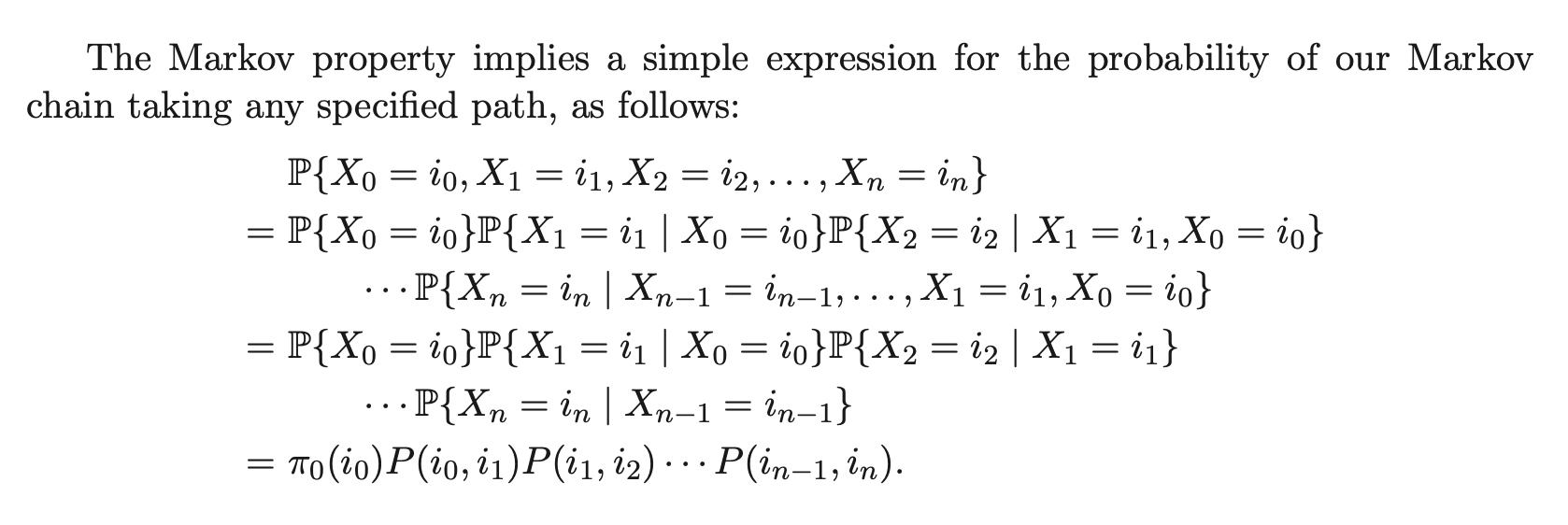
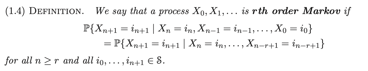
(i.e., dependent on the last r states)

1.3 Matrices

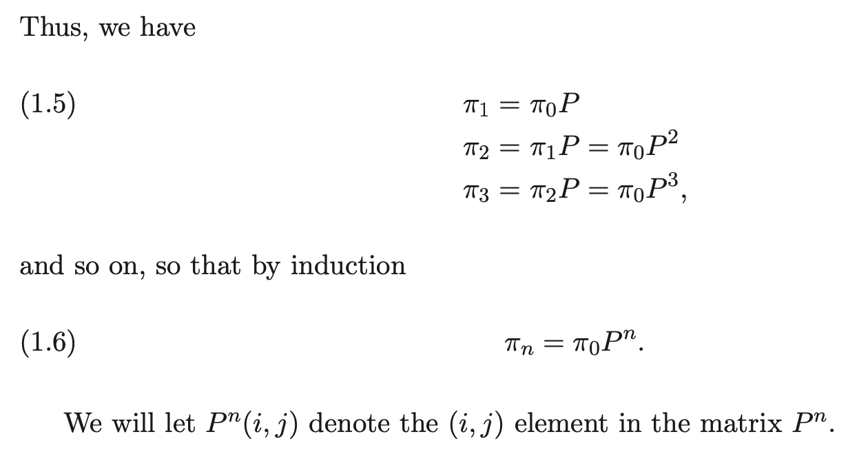
recall $\pi_0$ from 1.1. let $\pi_n$ denote the distribution of the chain at time $n$ analogously, $\pi_n(i) = \mathbb{P}\{X_n = i\}$. consider both as row vectors.

suppose that the state space is finite: $S = \{1, …, N\}$. by LOTP,

$$\pi_{n+1}(j) = \mathbb{P}\{X_{n+1} = j\} \newline = \sum_{i=1}^{N}\mathbb{P}\{X_n=i\}\mathbb{P}\{X_{n+1} = j | X_n=1\} \newline \sum_{i=1}^{N} \pi_n(i)P(i,j) = \pi_{n+1} = \pi_nP.$$

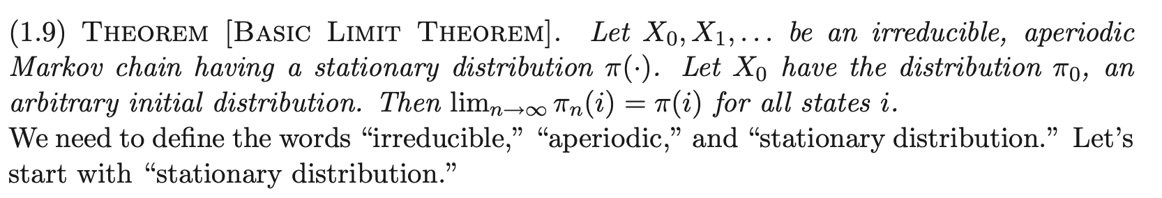
1.4 Basic Limit Theorem of Markov Chains

1.5 Stationary Distribution

stationary distribution amounts to saying $\pi = \pi P$ is satisfied, i.e.,

$$\pi(j) = \sum_{i \in S} \pi(i) P(i,j)$$

for all $j \in S$.

a Markov chain might have no stationary distribution, one stationary distribution, or infinitely many stationary distributions.

for subsets $A, B$ of the state space, define the probability flux from set $A$ into $B$ as

$$\text{flux}(A, B) = \sum_{i \in A} \sum_{j\in B} \pi(i) P(i,j)$$

1.6 Irreducibility, Periodicity, Recurrence

Use $\mathbb{P}_i(A)$ as shorthand for $\mathbb{P}\{A | X_0 = i\}$, and same for $\E_i$.

Accessibility: for two states $i, j$, we say that $j$ is accessible from $i$ if it is possible for the chain ever to visit state $j$ if the chain starts in state $i$:

$$\P_i \{\cup_{n=0}^{\infty} \{X_n = j\} \} > 0.$$

Equivalently,

$$\sum_{n=0}^{\infty}P^n (i, j) = \sum_{n=0}^{\infty}\{X_n = j \} > 0.$$

Communication: we say $i$ communicates with $j$ if $i$ is accessible from $j$ and $j$ is accessible from $i$.

Irreducibility: the Markov chain is irreducible if all pairs of states communicate.

The relation “communicates with” is an equivalence relation; hence, the states space $S$ can be partitioned into “communicating classes” or “classes.”

–

The Basic Limit Theorem requires irreducibility and aperiodicity (see 1.5). Trivial examples why:

• Irreducibility: takes $S = \{0,1\}, P = \begin{pmatrix} 1 & 0 \\ 0 & 1 \end{pmatrix}$. Then $\pi_n = \pi_0$ holds for all $n$, i.e., $\pi_n$ does not approach a limit independent of $\pi_0$.
• Aperiodicity: same $S$, take $P = \begin{pmatrix} 0&1 \\ 1&0 \end{pmatrix}$. If, for example, $\pi_0 = (1,0),$ $\pi_n$ alternates with even and odd $n$, and does not converge to anything.

–

Period: Given a Markov chain $\{ X_0, X_1, ... \}$, define the period of a state $i$ to be the greatest common divisor

$$d_i = \text{gcd} \{n : P^n (i, i) > 0 \}.$$

THEOREM: if the states $i$ and $j$ communicate, then $d_i = d_j$.

The period of a state is a “class property.” In particular, all states in an irreducible Markov chain have the same period. Thus, we can speak of the period of a Markov chain if the Markov chain is irreducible.

An irreducible Markov chain is aperiodic if its period is $1$, and periodic otherwise. (A sufficient but not necessary condition for an irreducible chain to be aperiodic is that there exists a state $i$ such that $P(i,i) > 0$.)

–

One more concept for the Basic Limit Theorem: recurrence. We will begin with showing recurrence, then showing that it is a class property. In particular, in an irreducible Markov chain, etiher all states are recurrent OR all states are transient.

The idea of recurrence: a state $i$ is recurrent if, starting from the state $i$ at time 0, the chain is sure to return to $i$ eventually. More precisely, define the first hitting time $T_i$ of the state i by

$$T_i = \inf \{n>0 : X_n = i \}.$$

Recurrence: the state $i$ is recurrent if $\P_i \{ T_i < \infty \} = 1$. If $i$ is not recurrent, it is called transient.

(note that accessibility could be defined: for distinct states $i \neq j$, $j$ is accessible from $i$ iff $\P_i \{ T_j < \infty \} > 0$.)

THEOREM: Let $i$ be a recurrent state, and suppose that $j$ is accessible from $i$. Then all of the following hold:

• $\P_i \{T_j < \infty \} = 1$
• $\P_j \{T_i < \infty \} = 1$
• The state $j$ is recurrent

–

We use the notation $N_i$ for the total number of visits of the Markov chain to the sate $i$:

$$N_i = \sum_{n=0}^{\infty} I \{X_n = i \}.$$

THEOREM: The state $i$ is recurrent iff $\E_i(N_i) = \infty.$

COROLLARY: If $j$ is transient, then $\lim_{n \rightarrow \infty} P^n(i,j) = 0$ for all states $i$.

–

Introducing stationary distributions.

PROP: Suppose a Markov chain has a stationary distribution $\pi$. If the state $j$ is transient, then $\pi(j) = 0$.

COROLLARY: If an irreducible Markov chain has a stationary distribution, then the chain is recurrent.

Note that the converse for the above is not true. There are irreducible, recurrent Markov chains that do not have stationary distributions. For example, the simple symmetric random walk on the integers in one dimension is irreducible and recurrent but does not have a stationary distribution. By recurrence we have $\P_0 \{T_0 < \infty \} = 1$, but also $\E_0 \{T_0 \} = \infty$. The name for this kind of recurrence is null recurrence, i.e., a state $i$ is null recurrent if it is recurrent and $\E_i(T_i) = \infty$. Otherwise, a recurrent state is positive recurrent, where $\E_i (T_i) < \infty$.

Positive recurrence is also a class property: if a chain is irreducible, the chain is either transient, null recurrent, or positive recurrent. In fact, an irreducible chain has a stationary distribution iff it is positive recurrent.

1.7 Coupling

Example of coupling technique: consider a random graph on a given finite set of nodes, in which each pair of nodes is joined by an edge independently with probability $p$. We could simulate a random graph as follows: for each pair of nodes $i, j$ generate a random number $U_{ij} \sim U[0,1]$, and join nodes $i$ and $j$ with an edge if $U_{ij} \leq p$.

How do we show that the probability of the resulting graph being connected is nondecreasing in $p$, i.e., show that for $p_1 < p_2$,

$$\P_{p1} \{ \text{graph connected}\} \leq \P_{p2} \{ \text{graph connected} \}.$$

We could try to find an explicit function for the probability in terms of $p$, which seems inefficient. How to formalize the intuition that this seems obvious?

An idea: show that corresponding events are ordered, i.e., if $A \subset B$ then $\P A \leq \P B$.

Let’s make 2 events by making 2 random graphs, $G_1, G_2$ on the same set of nodes. $G_1$ is constructed by having each possible edge appear with prob $p_1$, and for $G_2$, each edge present with prob $p_2.$ We can do this by using two sets of $U[0,1]$ random variables: $\{U_{ij}\}, \{V_{ij}\}$ for the first and second graph, respectively. Is it true that

$$\{G_1 \text{ connected}\} \subset \{G_2 \text{ connected} \}?$$

No, since the two sets of r.v.s are independently generated.

A change: use the same random numbers for each graph. Then

$$\{G_1 \text{ connected}\} \subset \{G_2 \text{ connected} \}$$

becomes true. This establishes monotonicity of the probability being connected.

Conclusion: what characterizes a coupling argument? Generally, we show that the same set of random variables can be used to construct two different objects about which we want to make a probabilistic statement.

1.8 Proof of Basic Limit Theorem

The Basic Limit Theorem says that if an irreducible, aperiodic Markov chain has a stationary distribution $\pi$, then for each initial distirbution $\pi_0$, as $n \rightarrow \infty$ we have $\pi_n (i) \rightarrow \pi(i)$ for all states $i$.

(Note the wording “a stationary distribution”: assuming BLT true implies that an irreducible and aperiodic Markov chain cannot have two different stationary distributions)

Equivalently, let’s define a distance between probability distributions, called “total variation distance:”

DEFINITION: Let $\lambda$ and $\mu$ be two probability distributions on the set $S$. Then the total variation distance $|| \lambda - \mu ||$ is defined by

$$|| \lambda - \mu || = \sup_{A \subset S} [ \lambda(A) - \mu(A) ].$$

PROP.: The total variation distance may also be expressed in the alternative forms

$$|| \lambda - \mu = \sup_{A \subset S} [ \lambda(A) - \mu(A) ] = \frac{1}{2} \sum_{i \in S} | \lambda(i) - \mu(i) | = 1 - \sum_{i \in S} \min \{ \lambda(i), \mu(u) \}.$$

We now introduce the coupling method. Let $Y_0, Y_1, ...$ be a Markov chain with the same probability transition matrix as $X_0, X_1, ...$, but let $Y_0$ have the initial distribution $\pi$ and $X_0$ have the initial distribution $\pi_0$. Note that $\{ Y_n \}$ is a stationary Markov chain with distribution $\pi$ for all $n$. Let the $Y$ chain be independent of the $X$ chain.

We want to show that, for large $n$, the probabilistic behavior of $X_n$ is close to that of $Y_n$.

Define the coupling time $T$ to be the first time at which $X_n = Y_n$:

$$T = \inf \{ n : X_n = Y_n \}.$$

LEMMA: For all n we have

$$|| \pi_n - \pi || \leq \P \{ T > n \}.$$

Hence we need only show that $\P \{T > n \} \rightarrow 0$, or equivalently, that $\P \{ T < \infty \} = 1.$

Consider the bivariate chain $\{ Z_n = (X_n, Y_n) : n \geq 0 \}.$ $Z_0, Z_1, ...$ is clearly a Markov chain on the state space $S \times S$. Since the $X$ and $Y$ chains are independent, the probability transition matrix $P_Z$ of chain $Z$ can be written

$$P_Z (i_x i_y, j_x j_y) = P(i_x , j_x) P(i_y, j_y).$$

$Z$ has stationary distribution

$$\pi_Z (i_xy i_y) = \pi(i_x) \pi(i_y).$$

We want to show $\P \{ T \leq \infty \}.$ So, in terms of the $Z$ chain, we want to show that with probability one, the $Z$ chain hits the “diagonal” $\{ (j,j) : j \in S\}$ in $S \times S$ in finite time. To do this, it is sufficient to show that the $Z$ chain is irreducible and recurrent.

1.9 SLLN for Markov Chains

Ch. 2 – Markov Chains: Examples & Applications

Ch. 3 – MRFs and HMMs

Ch. 4 – Martingales

Ch. 5 – Brownian Motion

Ch. 6 – Diffusions and Stochastic Calculus

Ch. 7 – Likelihood Ratios

Ch. 8 – Extremes and Poisson Clumping