Geometric and Topological Methods in ML

Notes and relevant papers / readings for geometric and topological methods in machine learning. IN PROGRESS.

2. Geometric graphs, construction, clustering

Basics: metric spaces / metrics, graphs. Geometric graphs have vertices as points in a metric space, with edges defined by low distances in the metric space.

kNN, $\epsilon$-NN graphs. kNN construction via KD tree.

Shortest paths methods: Dijkstra’s (single source, $O(|E| + |V|\log |V|)$ Floyd Warshall (all pairs, $O(|V|^3)$

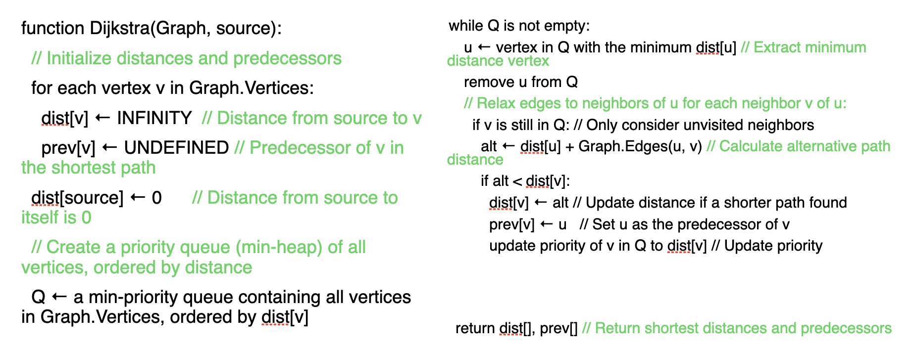
Dijkstra:

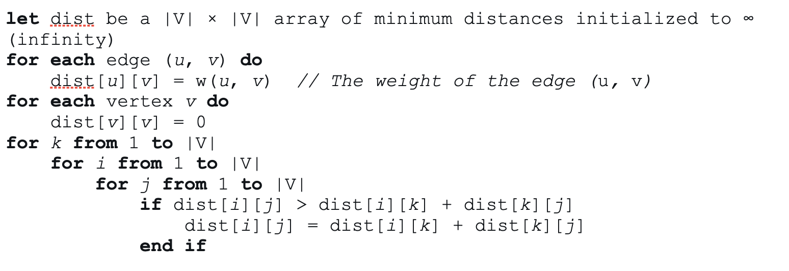
Floyd Warshall:

We are usually interested in using shortest paths to mimic geodesic distances. Also, Alamgir (ICML 2012) shows us that unweight 1-NN graphs lead us to weird paths (want to make least number of hops, so sometimes tends towards sparse areas of great distance in the metric), and that weighted distance converges to the length of the shortest path connecting two nodes.

Manifold learning based graph construction

Distance is converted to affinities via kernels (e.g. Gaussian kernel):

$$\text{affinity}_{i,j} = \exp \left( - \frac{\text{dist}(x_i, x_j)^2}{2 \sigma^2} \right).$$

The process usually goes data $\rightarrow$ calculate distances $\rightarrow$ calculate affinities.

Graph-based clusters / community detection

Hierarchical clustering:

• Link neighbors
• Link clusters

How do we measure distance between clusters? There are a couple of methods: single, average, and complete linkage. We can think of single linkage as linking the two closest points between two clusters, complete as linking the furthest, and average as linking the average. Single linkage is most common:

• start with every point in its own cluster
• merge the two closest clusters
• recompute distances based on min distance to the newly formed cluster
• repeat

Modularity

$A_{ij}$ is the actual affinity between $i,j$.

$P_{i,j}$ the probability of an edge existing between $i,j$, calculated by:

• generate random edges of the same degrees
• then the prob is $k_i * k_j / 2m$, where $m$ is the total number of edges in the graph.

Modularity is the sum of $A_{ij} - P_{ij}$ overall:

$$Q = \frac{1}{2m} \sum_{i,j} (A_{ij} - \frac{k_i k_j}{2m}) \delta(c_i, c_j)$$

Modularity optimization: Louvain used to be standard, now most use Leiden. Louvain has two phases:

• Finding communities:
  • Consider each node individually
  • See if the node should be moved into a neighboring community: select the community with the greatest change in modularity. If moving it corresponds with a positive change in modularity, move it.
  • Check only $K$ neighbors of the node
• Coarse graining:
  • Each community in phase 1 becomes a node in phase 2
  • Repeat phase 1

Why do we care about modularity? Based on its definition, we can think of it as a measure of the strength of a graph into modules / groups / communities. Networks with high modularity have dense connections between nodes within modules but sparse connections between nodes in different modules.

Recommended reading

• Alamgir et al. Shortest Path Distances in k-nearest Neighbor Graphs, ICML 2012
• Lishan et al., Data-driven graph construction and graph learning: A review, Neurocomputing 2018
• Kd-trees (Wikipedia)
• Dijkstra’s algorithm (Wikipedia)
• Floyd Warshall algorithm (Wikipedia)
• Newman, Modularity and community structure in Networks, PNAS 2006
• Blondell et al. Fast unfolding of communities in large networks, Journal of Statistical Mechanics: theory and experiment, 2008

3. Data diffusion, diffusion maps, spectral clustering

Representation Learning

We want to find the “best” representation of our data; i.e., we want to preserve as much information as possible while obeyind some penalty that simplifies the representation.

What kind of information should be preserved, and how do we define “simple”?

• Low-dimensional
• Sparse
• Independent components

These criteria aren’t necessarily mutually exclusive. Simple representations are good for interpretability (visualization), reducing computational cost (compression), and performance on supervised tasks (can be easier to classify / regress from).

Isomap (Tenanbaum, 2020)

• Construct neighborhood graph
• Find all pairs shortest paths
• Apply MDS to compute low-dimensional coordinates that preserve distances

MDS (Multidimensional Scaling)

MDS finds an embedding of the data that preserves distances by optimizing point positions such that “stress” is minimized:

$$\text{stress}_{D} (x_1, x_2, ..., x_N) = \sqrt{ \sum_{i \neq j = 1, ..., N} (d_{ij} - ||x_i - x_j || )^2 }.$$

This can be done with gradient descent and other related procedures.

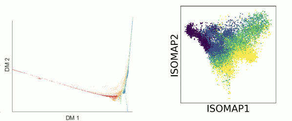
Isomap’s weakness: real data is often very noisy, and the shortest path algorithm results in noisy distances between points. More commonly, we might see UMAP being used or PHATE (geometry preserving, common in biology).

Diffusion maps

Diffusion distance can be more robust to noise! Introduced by Coifman and Lafon. 3 step process:

• Compute affinities with Gaussian kernel
• Compute degree matrix
• Markovian diffusion operator gives us coordinates

1. Recall kernel functions (discussed previously for converting distances to affinities). If $(X, A, \mu)$ is a measurable space, a kernel function is a mapping $K : X \times X \rightarrow \R$ such that for any $x, y \in X,$

$$\begin{align*} K(x,y) &= K(y,x) \\ K(x,y) &\geq 0. \end{align*}$$

Kernels are generally nonlinear. Diffusion maps are specifically defined with respect to the Gaussian kernel:

$$k(x,y) = e^{-||x-y||^2 / \eps},$$

where $\eps$ is a bandwidth parameter. This kernel captures a notion of affinity/similarity between points in $X.$

The Gaussian kernel emphasizes local connections and pushes non-local connections to $0$ in a “softer” way than kNN. We can also threshold these outputs for computational purposes (so that the affinity graph wouldn’t be fully connected).

2. After computing affinities with the Gaussian kernel, we define the degree matrix. For a weighted graph, the degree of vertex $x$ is defined as the sum of similarities/affinities between its neighbors:

$$q(x) = \sum_{i=0}^{i < n} k(x, v_i).$$

The degree matrix is a diagonal matrix where $d_{i,i} = q(\text{vertex } i)$.

3. We can now define the “diffusion operator”

$$P(x,y) = k(x,y) / q(x),$$

a matrix of transition probabilities with row-normalized affinities. Therefore, this matrix is Markov & describes a random walk over the data.

Since $P$ represents the 1-step transition probabilities, $P^t$ represents the $t$-step random walk probabilities.

The diffusion map representation is a spectral embedding; that is, $P$ has a spectral decomposition that we can use to assign coordinates in the embedding to each data point.

Consider the matrix $A$ where

$$a(x,y) = \frac{k(x,y)}{\sqrt{q(x)} \sqrt{q(y)}} = q(x)^{1/2} * p(x,y) * q(y)^{-1/2}.$$

Then $A = Q^{1/2}*P*Q^{-1/2}$ and is symmetric, so there exists an eigendecomposition. In fact, $P$ and $A$ are similar, so they must have the same eigenvalues and related eigenvectors.

Let the eigenvectors of $A$ be $\phi_1, \phi_2, ..., \phi_n$.

• A left eigenvector of $P$, $\psi_j$, would be $= Q^{-1/2}\phi_j$.
• A right eigenvector of $P$, $\Psi_j$, would be $= \phi_j Q^{-1/2}.$

We can use these eigenpairs are used to compute the spectral decomposition of $P$:

For $1 = \lambda_0 \geq \lambda_1 \geq \lambda_2 \geq ... \geq \lambda_\delta > 0,$

$$\begin{pmatrix} \phi_0 & \phi_1 & \phi_2 & \cdots & \phi_delta \end{pmatrix}$$

where each $\phi_i$ is a column eigenvector from $A$, we can map a datapoint $x$ to its embedding coordinates as:

$$x \mapsto \phi^t(x) = [ \lambda_0^t \phi_0(x), \lambda_1^t \phi_1(x), \lambda_2^t \phi_2(x), ..., \lambda_\delta^t \phi_\delta(x)]^T.$$

Properties of the spectrum

• Eigenvalues are in range $[0,1]$
• 1 is an eigenvalue
• The first eigenvector is the steady state/stationary vector $\phi_0$ of all 1’s
• Stationary distribution given as $\pi(y) = \frac{q(y)}{\sum_{z \in X} q(z)}$
• Markov chain is reversible, e.g. $\pi(x)p(x,y) = \pi(y)p(y,x)$

Powers of the matrix $A$ make lower eigenvalues get lower:

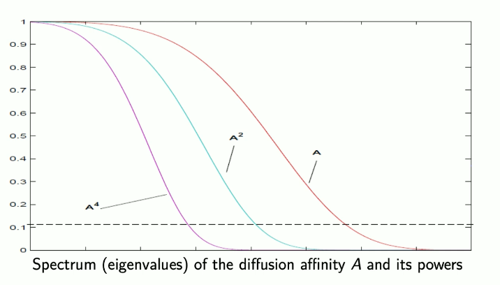
Hence powers of $A$ denoise in a low-pass filtering manner. When we map $x$ to its new coordinates, we can use only the first $k$ eigvals/eigvecs due to spectrum decay while still maintaining accuracy, which reduces our dimensionality.

Diffusion distance

Diffusion maps preserve diffusion distance, a family of $L^2$ distance on the transition probability distribution between 2 points:

$$D_t(x,y)^2 = ||p_t(x, \cdot) - p_t(y, \cdot) ||^2_{L^2(X, d\mu / \pi)}.$$

This is essentially the Euclidean distance between rows of the diffusion operator.

Diffusion distance can also be interpreted as the overall distance in walking probabilities after $t$ steps when starting out in point $x$ vs. point $y$.

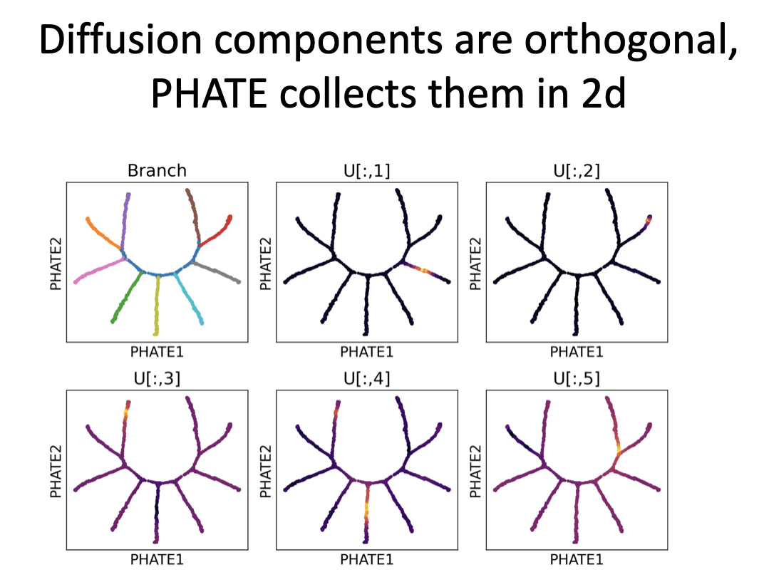
Diffusion maps do a good job at cleaning data, but are not necessarily great at visualization. This is partially because diffusion maps split information into multiple orthogonal directions, e.g. plotting in 2-D will likely only show us 2-ish trajectories.

Partitioning data with K-means

In k-means, we want to find $k$ splits/partitions to minimize variance within each cluster:

• initialize: pick $k$ random cluster centroids
• assignment: assign each datapoint $x_i$ to cluster $S_j$ that has the nearest mean $\mu_j$
• update: compute the means of clusters $\mu_i = \frac{1}{|S_i|} \sum_{x_j \in S_i} x_j$

k-means converges because each reassignment lowers the MSE:

$$\argmin_S \sum_{i=1}^k \sum_{x \in S_i} || x- \mu_i ||^2 = \argmin_S \sum_{i=1}^k |S_i|\text{var}(S_i).$$

Therefore, this optimization will reach a local minima. However, k-means only works well on data with certain characteristics. It assumes:

• k is chosen correctly
• data is distributed normally around the mean
• clusters all have equal variance
• clusters all have the same number of points

It is also sensitive to initialization and outliers.

An alternative is spectral clustering. Spectral clustering can use eigenvectors of the diffusion oeprator or Laplacian. Advantages of using the spectrum for k-means:

• good for clusters of arbitrary shape
• good for graph data
• only need connectivity data

How it works:

• construct a similarity graph
• compute diffusion operator or graph Laplacian
• using top k eigenvectors, run k-means

Recommended reading

• Nadler et al., Diffusion maps, spectral clustering, and eigenfunctions of Fokker-Planck operators, NeurIPS 2005
• Coifman and Lafon, Diffusion Maps, Applied and computational harmonic analysis 2006
• Tenenbaum et al., A global geometric framework for non-linear dimensionality reduction, Science 2000 (Isomap)

4. Data diffusion, continuous diffusion, PHATE

Previously (3), diffusion maps.

Connections between discrete and continuous diffusion

For finite bandwidth $\epsilon$, the Markov chain in discrete time and space converges to a Markov process in discrete time but continuous space.

As $\epsilon \rightarrow 0$, this jump process converges to a diffusion process on $\R^n$. In the continuum limit of infinitely many points and continuous time, this resembles a Fokker-Planck diffusion process.

Fokker-Planck Diffusion Process

Describes diffusion as a mix of random Brownian forces $W_t$ and drag forces $U(x)$:

$$dX_t = \mu (X_t, t) dt + \sigma (X_t, t) dW_t.$$

Given an initial condition at time $s < t$ this follows the forward Fokker-Planck equation (FPE):

$$\frac{\partial p}{\partial t} = \nabla \cdot (\nabla p + p \nabla U(x)).$$

$\Delta$ refers to the Laplacian $\Delta y = \nabla(\nabla u)$, the divergence of the gradient.

General solutions of the FPE are given by the eigenfunctions of the FPE operator. In our case, the potential is the log of the data density (so drag is related to data density).

Data density

The density of the data $D(x_i) = q(x_i) = \sum_j A(x_i, x_j)$ is a proxy for the density at point $x_i$.

In the setting of our data, the “potential” $U$ is the log of data density:

$$U(x) = - \log (q(x)).$$

Essentially, the FPE is saying we have a diffusion process that has “drag” because of data density.

Anisotropic normalization

Instead of the diffusion kernel before, we can define a different symmetric kernel $M_S = D^{ - \alpha} A D^{- \alpha}$:

$$M_S = \frac{k(x,y)}{q(x)^\alpha q(y)^\alpha}.$$

If $\alpha=1$ this kernel has uniform degree (all points have density of 1).

Convergence to Laplace-Beltrami

If you set $\alpha =1$, then $U = \log(1) = 0$. Then the second term in the FPE drops out:

$$\frac{\partial p}{\partial t} = \nabla \cdot (\nabla p + p \nabla U(x))$$

and we are left with

$$\frac{\partial p}{\partial t} = \nabla p$$

which is purely controlled by the Laplacian. This is a second derivative operator and purely geometric, hence separating density from geometry.

Summary: In infinitely many points and continuous time the FPE represents the diffusion process. We need to reconcile with the drag term $U$ in the FPE, which is given by the density of the data. We resolve this by dividing it out in anisotropic normalization kernel, which converges to the Laplace Beltrami operator, successfully separating density from geometry.

Application of diffusion maps to clustering / PHATE

Previously (3): k-means clustering algorithm, spectral clustering using diffusion map coordinates.

PHATE goal: Create a visualization that preserves data geometry in low dimensions.

• Denoise the data
• Capture geometry
• Compress into visualizable dimensions
• Allow for scalability to large modern datasets

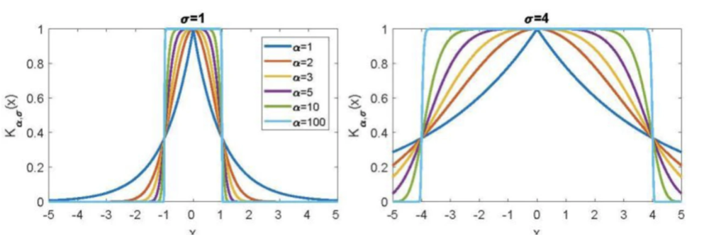
PHATE uses adaptive bandwidths/an alpha-decaying kernel:

$$K_{k, \alpha}(x,y) = \frac{1}{2} \exp \left( - \left( \frac{||x-y||_2}{\epsilon_k(x)} \right)^\alpha \right) + \frac{1}{2} \exp \left( - \left( \frac{||x-y||_2}{\epsilon_k(y)} \right)^\alpha \right),$$

where

• $\alpha$ controls rate of decay of kernel
• $\epsilon_K$ the distance to $k$-th nearest neighbor
  • $K$ a parameter
• adaptive bandwidths adjust for density.

Plot of alpha decay kernel:

Spectral entropy

• The amount of entropy, proxy for information, decays as $t$ increases
• Choose a spot after the elbow
• This heuristically corresponds to after the noise decays sand before signal decay

Potential distance in PHATE

• a triplet distance between $(x,y)$ that sums over diffusion inner products to all other points $z$
• damps diffusion probabilities using a log factor which increases the importance of far points $z$ in contextualizing $(x,y)$
• accounts for the covariance between random walks arising from $x$ vs those arising from $y$

Diffusion components track one branch at a time, zeroing out everything else. Makes them good for clustering but not great for visualization. See image for example:

Other remarks

• Ways to speed up PHATE: compressed diffusion
• DeMAP: denoised manifold affinity preservation
• PHATE preserves cluster and trajectory structure, denoises to reveal more local structure

Recommended reading

• Nadler et al., Diffusion maps, spectral clustering and reaction coordinates of dynamical systems, Applied and Computational Harmonic Analysis 2006
• Moon et al., Visualizing Structure and Transitions in High Dimensional Biological Data, Nature Biotechnology 2019

5. tSNE and UMAP

Ways to compare probability distributions

• cross entropy
• divergences
  • KL divergence
  • Jensen-Shannon divergence
• distances
  • Wasserstein distance
  • maximum mean discrepancy
  • more in (6)

Entropy

Represents the expected amount of uncertainty in a distribution:

$$H(P) = - \sum_i P(x_i)\log(P(x_i)).$$

Cross Entropy

Given 2 distributions $P,Q,$ how many bits on average does it take to “encode $Q$” in a code that is optimized for $P$?

$$H(P,Q) = - \sum_i Q(x_i) \log(P(x_i)).$$

Example: encoding a distribution $Q$.

If we have 3 outcomes $a, b, c$ and $q(a) = 1/2, q(b) = q(c) = 1/4,$ we can encode:

• a as 0
• b as 1
• c as 10

Then the average number of bits needed is

$$(1/2)*1 + (1/4)*1 + (1/4)*2.$$

Suppose we use encoding for $Q$ on a distribution $P$ now, where $p(a) = p(b) = 1/4$ and $p(c) = 1/2$. Then the average number of bits needed is

$$(1/4)*1 + (1/4)*1 + (1/2)*2.$$

KL divergence

The expected number of extra bits needed if using samples from $P$ on a code optimized for $Q$. This is related to cross entropy and sometimes called relative entropy:

$$D_{KL}(P||Q) = - \sum_i P(x_i)\log \left( \frac{P(x_i)}{Q(x_i)} \right) = \sum_i P(x_i)\log \left( \frac{Q(x_i)}{P(x_i)} \right).$$

Note that

$$D_{KL}(P||Q) = H(P,Q) - H(P).$$

Important properties: $D_{KL}(P||Q)$ is not a distance. It is not the same as $D_{KL}(Q||P)$ and does not follow the triangle inequality.

Jensen Shannon Distance

JS divergence is symmetric but still does not follow the triangle inequality. Can be made a proper distance by taking a square root of the Jensen Shannon divergence.

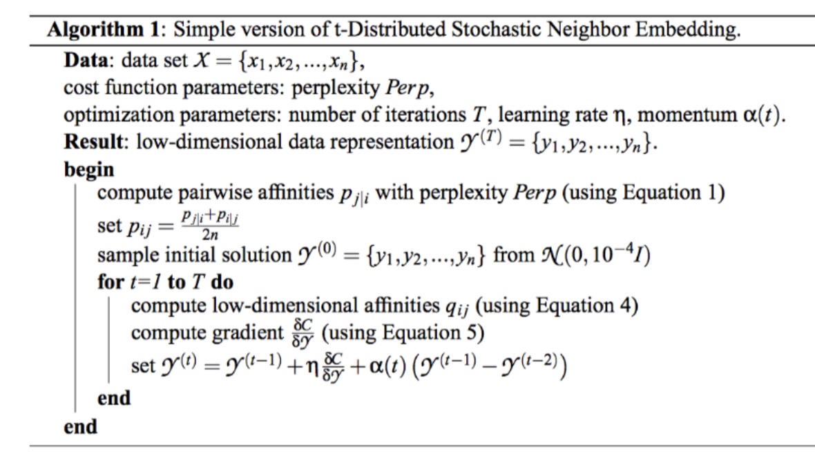
tSNE: t-Stochastic Neighbor Embedding

Concept: Maintain neighborhoods, preserve the data’s shape both locally and globally.

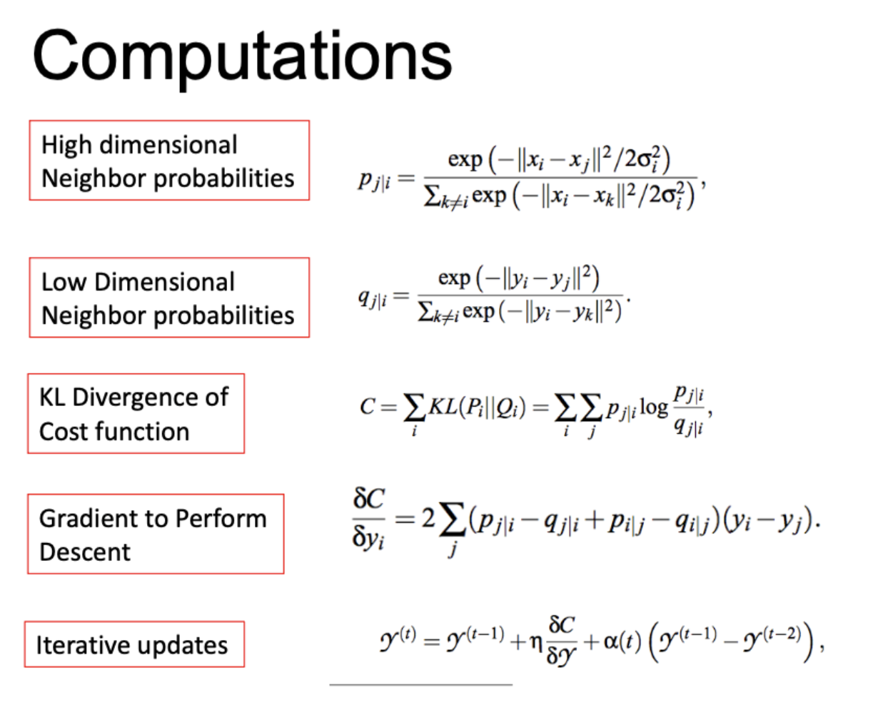
Stochastic neighbors: tSNE creates a probability distribution that represents similarities between neighbors, or the conditional probability that one node would pick another as its neighbor. The similarity for a node $x_i$ is defined to be proportional to a probability density under a Gaussian centered at $x_i$.

The variance (bandwidth parameter) for each of these Gaussians of any point $x_i$ is set to $\sigma_i$ such that the Shannon entropy of neighbors is a fixed value.

$$H(p(x_i, \cdot)) = - \sum_j p(x_i, x_j) \log(p(x_i, x_j)).$$

$$\text{perplexity} = W^{H(p(x_{i, \cdot}))} = \text{ effective no. of nbrs}$$

This fixed value is defined by a parameters we set called perplexity.

Penalty: tSNE minimizes KL divergence, i.e., we want to match the probability distributions of high dimensional and low dimensional neighbors. Optimize with SGD.

Note on SNE vs tSNE: high-dimensional similarities are measured as shown below and use an adaptive bandwidth. The low-dim similarities are computed differently depending on if using SNE or tSNE.

In both SNE and tSNE, we are moving points around to minimize KL divergence. However, the problem with normal SNE is that there is a low penalty for moving points (in low dim) around if they are far away in high dimensions.

To fix this, tSNE uses the student-t distribution in low-dim space. The fatter tails help keep $p_{i,j}$ a little bit higher, so points which are far away can still be reasonably penalized in their low-dim representations. This also helps with crowding.

UMAP

Uniform Manifold Approximation and Projection = UMAP.

Assumes:

• the data is uniformly distributed on Riemannian manifold
• Riemannian metric is locally constant
• manifold is locally connected

Effectively uses a tSNE-like method to embed data.

• UMAP works with unnormalized similarities
• uses the same adaptive kernel as tSNE
• symmetricized high dimensional similarities on kNN:

$$\mu_{i \rightarrow j} = \begin{cases} \exp( - (d(x_i, x_j) - d(x_i, x_{i_1}))/ \sigma_i) & \text{ for } j \in \{i_1, ..., i_k\} \\ 0 & \text{ else.} \end{cases}$$

$$\mu_{ij} = \mu_{i \rightarrow j} + \mu_{j \rightarrow i} - \mu_{i \rightarrow j}\mu_{j \rightarrow i} \in [0,1].$$

• low dimensional similarities

Uses binary crossentropy loss, a penalty for modeling similar points as dissimilar and vice versa:

$$\mathcal{L} ( \{e_i \} | \{ \mu_{ij}\}) = -2 \sum_{1 \leq i < j \leq n} \mu_{ij} \log(v_{ij}) + (1 - \mu)_{ij} \log(1 - v_{ij}).$$

Initialization to a Laplacian eigenmap (Belkin and Niyogi), a geometric method. The “effective” loss function says that UMAP effectively binarizes neighbors.

Scalability: neighbors and non-neighbors are just sampled from the data graph. Therefore, we don’t have to compute a whole affinity matrix or Markov matrix like in tSNE, hence it is much faster and more scalable.

Attraction-repulsion continuum: Unlke tSNE, something being close doesn’t mean something else has to be far (effect of row-stochastic normalization). Therefore, UMAP visualizations have a less “explosive” look:

UMAP vs tSNE

• UMAP uses similarities, tSNE uses probabilities (stochastic nbrs)
• positive sampling of neighbors vs. negative sampling of non-neighbors
• Laplacian eigenmap initialization of UMAP is important and different

Recommended reading

• Hinton & Roweis, Stochastic Neighbor Embedding, NeurIPS 2002
• van der Maaten, Laurens, and Geoffrey Hinton. “Visualizing Data using t-SNE.” Journal of Machine Learning Research 9 (2008):
• Bohm et al. Attraction-Repulsion Spectrum in Neighbor Embeddings, JMLR 2022
• Damrich & Hamprecht, On UMAPs True Loss Function, NeurIPS 2025

6. Graph Laplacians and Graph Signal Processing

Laplacian

Laplacian = divergence of the gradient, sum of all the unmixed second derivatives at any point.

$$\Delta f = \nabla \cdot (\nabla f) = \nabla^2 f = \frac {\partial^2 f}{\partial x^2} + \frac{\partial^2 f}{\partial y^2} + \frac{\partial^2 f}{\partial z^2}.$$

In 1-D, Laplacian is the second derivative, which measures the curvature of a function. In multiple dimensions, the Laplacian at a point measures how much the function’s value deviates from the average ofits values in a small neighborhood around that point, related to mean curvature.

The heat equation uses the Laplacian:

$$\frac{\partial u}{\partial t}$$

to represent the rate at which a quantity diffuses at a given point. Other applications of the Laplacian include computer vision, quantum mechanics (Hamiltonian), electromagnetism (Poisson eq.).

The Laplacian is a linear operator:

• $\Delta(f+g) = \Delta f + \Delta g,$ additivity
• $\Delta [cf] = c \Delta f,$ homogeneity

$\cos(\omega x), \sin(\omega x)$ are eigenfunctions of the Laplacian in Euclidean space (e.g., the second deriv of each function is a scalar multiple of the og. function).

Discrete and Graph Laplacian

A discrete Laplacian is a discrete analog of continuous Laplacians, often on a grid. In a graph, the Laplacian operator is a linear operator acting as a matrix that represents how a function’s value at a vertex differs from its average over neighboring vertices in a graph. Therefore, the graph Laplacian is defined as the degree matrix minus the adjacency matrix

$$L = D- A,$$

which measures how a vertex is different from its neighbors.

Quick note on finite difference approximation, where continuous second-order partial derivatives of the Laplacian are replaced iwht finite difeerences using Taylor series expansions, eg:

$$\frac{\partial^2 u}{partial x^2} \approx \frac{u(x+h, y) - 2u(x,y) + u(x-h,y)}{h^2}.$$

• Unnormalized Laplacian $L = D - A.$

• Normalized Laplacian $L = I - D^{-1/2} A D^{-1/2}.$

• Random walk Laplacian $L = I - D^{-1} A = I - M,$ related to Markovian matrix.

We can think of the graph Laplacian as a discrete version of finite difference approximation.

By the spectral theorem, $L$ is eigendecomposable into orthonormal eigenbasis $L = U \Lambda U^T,$ where $LU_0 = \lambda_0 U_0, LU_1 = \lambda_1 U_1, ....$

Eigenvalues of $L$ are in the range of $0 \leq \lambda_0 \leq \lambda_1 \leq ... \leq \lambda_n$.

We often take $L$ to be a normalized Laplacian $L = I - D^{-1/2}AD^{-1/2},$ which helps remove the effect of density.

$0$ is an eigenvalue of the eigenvector $(1, 1, 1, \cdots).$ The second smallest eigenvalue, called the “Fiedler value,” measures graph connectivity.

Laplacian Eigenmaps

Belkin & Niyogi, maps each point to its Laplacian eigenvector coordinates.

$$x_i \rightarrow U_1(x_i), U_2(x_i), ..., U_k(x_i)$$

where each $U_i$ an eigenvector of $L= D-K$. ($x_i$ literally gets mapped to the $i$-th coordinate in each eigenvector, using the num. of eigenvecs depending on the dimension you’re reducing to.)

We can recast this as a smoothness minimization problem: a desirable embedding may be one where nearby points are similar. We choose a Gaussian kernel $K(x_i, x_j) = \exp{-||x_i - x_j||^2 / \epsilon}.$

$$C(Y) = 1/2 \sum_{i,j} (y_i - y_j)^2 K(x_i, x_j) = y^t L y.$$

Based on Courant-Fisher, the minimizer of this is $U_0$ and the next best minimizer is $U_1$.

Graph Signal Processing

Fourier transform of a signal:

$$f(k) = \int_{-\infty}^{\infty} f(x) e^{-2 \pi i k x}dx.$$

Usually, we don’t have the functional form available to compute the integral, so we have to use discrete samples and discrete wavelengths for the discrete Fourier transform.

DFT is a matrix multiplication:

We can interpret features as signals on a graph. Applying graph Fourier transform, $L = U \Lambda U^T$, we can decompose signals into graph Fourier coefficients.

Spectral Graph Filtering

Introduced by Stankovic et al. 2018. Interested in finding which frequencies are noise, then altering the frequencies to retrieve the corrected signal.

Filter is generally constructed by having some function $H$, which changes the eigenvalues $H(\lambda_i)$ (see below).

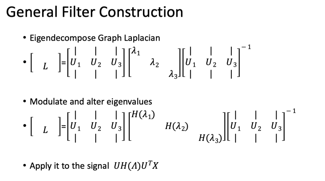
Data signals are low frequency and noise can be high frequency. We can take noise off by taking high frequency eigenvectors off. A low pass filter is when you let low frequencies through and filter out high frequencies.

Problems with frequency domain filters:

• Problem 1: The filters are not localized operations
  • They are operating globally based on frequency characteristics
  • Potential fix: Use wavelet filters instead of Fourier
    • Wavelets are localized in time and space
• Problem 2: Fourier transform is expensive, eigendecomposition of an NxN matrix each time
  • Fix: Polynomial filters (will cover in GNN lecture)
  • Fix: Diffusion based operations (also a polynomial filter)

K-filter coefficients

Reduce number of coefficients in filter

Chebyshev Polynomials

Use polynomial filter, automatically applies filter to eigenvalues and not eigenvectors.

From Fourier to Wavelets

• Fourier transforms capture global frequency information, frequencies that persist over the entire length of the signal
• What about small bursts of frequency changes?
• Uneven frequency distributions over time?
• These might benefit from a more localized frequency domain analysis

A solution: wavelets! Unlike a sine or cosine function, a wavelet is a localized oscillation. THey can be scaled (to look at low vs high frequency components) and translated (to look at different times and locations).

Discrete wavelet transform

Diffusions can be used to create wavelets. Diffusion wavelets , formed by taking differences between two scales of diffusion.

Recommended reading

• Belkin and Niyogi Laplacian Eigenmaps for Dimensionality Reduction and Data Representation, Neural Computation 2003
• Shuman et al. The Emerging Field of Signal Processing on Graphs: Extending High-Dimensional Data Analysis to Networks and Other Irregular Domains
• Coifman & Maggioni, Diffusion Wavelets, Applied and Harmonic Analysis 2006
• Gao et al. Geometric Scattering for Graph Data Analysis, ICML 2019
• Castro et al. Uncovering the Folding Landscape of RNA Secondary Structure with Deep Graph Embeddings, IEEE Big Data 2019

7. Graph Neural Networks and Geometric Scattering

Rough neural network overview. COvered:

• neurons as linear transformation + nonlinear activation function
• differentiability of neural networks allows us to learn relationship between input and desired output
• nodes arranged in layers to form deep networks
  • depth creates a composition of functions to learn complicated relationships / increase abstraction
• learning algorithms automatically tune the weights and biases
  • gradient descent

Design choices

• activation fn
• cost fn
• number and dimension of layers
• connection / dropout between layers
• regularization (layers, batching, etc)
• more

Graph neural network connection

• Spatial (vertex space) construction
  • apply same operator and move over graph space in some fashion
  • notion of locality based on neighbors of a node
• Spectral construction
  • define a convolutional operation in graph spectral space
  • use signal processing theoery to define filters in the graph Fourier domain
  • notion of locality based on global properties of the filter

Graph notation–adjacency matrix can be weighted, vertex features are graph signals.

Message passing: aggregate information from neighbors, update. There can be several message passing iterations. After $k$ iterations you get a latent embedding of node $u$: $z_u = h^{(K)}_u$.

Aggregation and update steps can involve trainable weight matrices.

We can train GNNs to do node, edge, graph, and signal level tasks. Common tasks were node/edge/graph tasks.

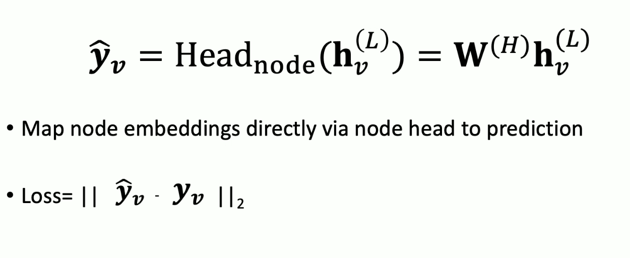
Node level tasks: node classification/regression. Map node embeddings directly via node head to prediction.

Link prediction: predict a link that should be there based on neighboring links.

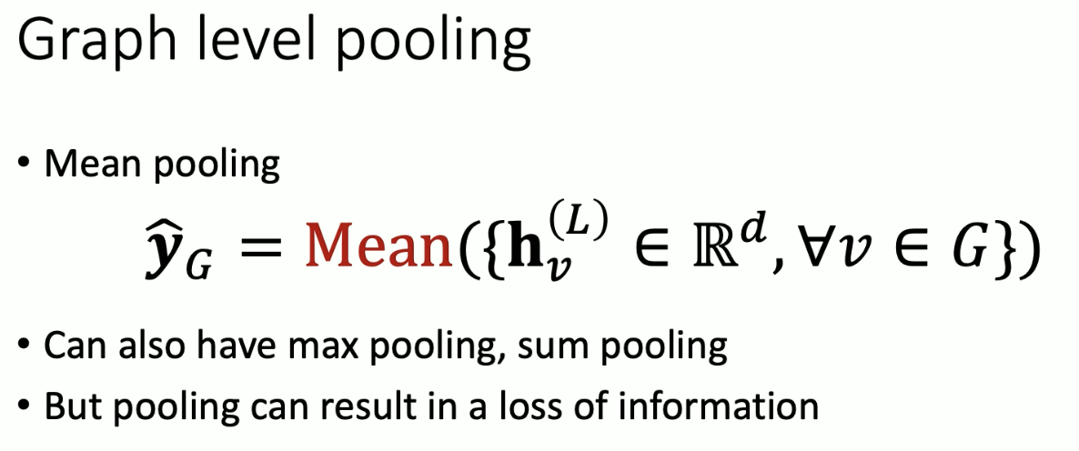
Graph level tasks: graph classification (does this graph have a 5-clique?). Graph regression (does the molecule this graph encodes bind to a virus?). Usually an additional layer of pooling. Also a pooling strategy called DiffPool.

Signal level task: features on vertices constitute a signal on a graph. Some graphs have more signals than vertices / edges. Classifying signals is largely unrecognized but important. Classic example is classifying traffic patterns.

1. Permutation equivariance: graph and node representations are the same regardless of how nodes are ordered in the adjacency matrix. Achieved via permutation equivariant aggregation operations like mmean, sum, max.

2. Inductive capability: sharing weights across nodes

These types of GNNs are limited and message passing can lead to oversmoothing.

Weisfeler Lehman Test of Isomorphism

Landmark result: GNNs are only as powerful as W-L test of isomorphism.

This test results in false positives (e.g. we can get graphs colored the same but aren’t isomorphic).

Some solutions

• Don’t just add layers to GNNs (eg message passing iterations): increase power with aggregation.
• Add skip connections–each layer does smoothing, so skip connections can be like a band pass.
• Feature augmentation / engineering
  • add features ot make GNNs more expressive, e.g. cycle count, node degree, edge degree, things from graph theory.

GraphSAGE

• inductive, message passing network
• mean aggregation (aggregates neighbors and concatenates self)
• LSTM aggregation

Spectral Construction

Features are signals on graph. These signals have an analogous Graph Fourier Transform, which involves using the eigenvectors of the graph Laplacian as waveforms (see previous lecs). Some spectral methods won’t directly compute GFT, will instead implement filter as polynomial of graph Laplacian.

See previous lec for Graph Laplacian review.

What does it mean to create filters?

We want to learn these filters with a neural network, which is what graph spectral nns were designed to do.

Problems

• fourier transform is expensive, requires eigendecomposition of $n \times n$ matrix each time
• fix: Chebyshev approximation instead
• many GCNs use first order polynomials of graph Laplacian (we learn the polynomial coefficients)

Wavelet-based constructions

See previous lec on continuous and discrete wavelet transforms (don’t need to know). Waveform centered at every node performs message aggregation.

Graph wavelet networks usually created with diffusion operator. Diffusion wavelets differ from lazy random walks (normal diffusion) because it tells you differences in diffusion between diadic powers.

Geometric Scattering

Alternative to GNNs. Use a cascade of diffusion wavelets to create a “deep” wavelet transform of a signal on a graph (instead of message aggregation and updating). The absolute values are pointwise non-linearity or “activation”. Cascade is parameterized by a scattering path that determines the scales of each wavelet.

Whole graph representation formed by taking an aggregation over all node level features.

8. Optimal Transport on Graphs

Recall KL, JS divergence–divergences have issues when distributions have disjoint support. Optimal transport–how hard is it to push/transform one distribution into another (Wasserstein)?

Wasserstein Distance & Optimal Transport

$$W_d(P,Q) = \inf_{\pi \in \prod(P,Q)} \int d(x,y) \pi(dx,dy)$$

Ground “cost” or distance:

$$d(x,y) = ||x-y||_2$$

(there’s also different $L^p$ Wasserstein dists.) Proportional to the amount of work needed to turn one dist into another.

Want to minimize

$$c = \sum_{(x,y)}P_{i,j}D_{i,j},$$

transport cost with constraints:

$$\sum_j P_{i,j} = r_i,$$

for $r_i$ the row marginal, and

$$\sum_i P_{i,j} = c_j,$$

with $c_j$ the column marginal. Linear program to optimize.

On Graphs

Distributions are normalized positive graph signals (if we have negative signal values, we can shift all signals to being positive).

Entropy Regularized Optimal Transport

$$\inf_{\pi \in \prod(P,Q)} \int d(x,y) \pi(dx,dy)^p \pi(dx,dy) - \epsilon h(\pi)$$

$$h(\pi) := - \int \log \pi d\pi.$$

Suppose you wanted to maximally spread the probability distribution.Then you might want to proportionally spread each bin in “source” distribution” $r(i)$ according to the needs of the sink distribution $c(j)$. This particular joint probability distribution is actually the independence table $rc^T$. This is the outer product of $r$ and $c$. Thus we can add a penalty for $P$ to deviate from the $rc^T$.

Discrete problem formulation with entropic constraint, solvable with Lagrange multipliers.

Sinkhorn

Primal method of optimal transport.

• Sinkhorn iteration algorithm $O(N)$ for optimal transport.
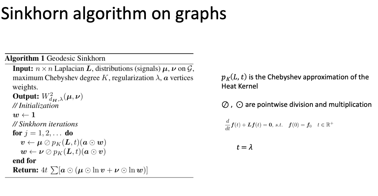
• Heat kernel method
  • Heat kernel on graph, given by matrix exponential approximated via Taylor series $H_t := e^{-tL}$ for $L$ the graph Laplacian
  • graph kernel can be used to implement sinkhorn on a graph
• Chebyshev polynomial approximation results in $K$ matrix-vector products, efficient for sparse matrices. $O(Kmn)$. Can be used to filter signal and begin sinkhorn iterations.
• Geodesic sinkhorn method: converts sinkhorn method to operate on a graph.

Dual form of optimal transport

Kantorovich Rubenstein Duality

Instead of finding ways to transport from one bin to another (primal), you try to find a signal whose likelihood is very different between two distributions:

In image, high likelihood with top dist. and low likelihood with low dist. Use multiscale historgrams/density estimates of the data:

• Take the difference of two histograms at different scales
• WEMD uses a wavelet basis to represent the difference histogram
• Since wavelets are a rich basis the wavelet transform is an approximation of f

This has also been done with trees (tree Wasserstein).

• sps you have data from 2 dists $P,Q$.
• combine the data and approx the data with a tree

Dual form computations vs primal

• Pros: faster, results from $L^1$ norms on data embeddings
• Cons: loss of accuracy and information. Limitations on ground distance (usually Euclidean), structural assumptions (image, tree embeddings).
• We want the best of both worlds, e.g. adapting to data structure, accurate, fast.

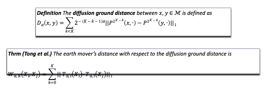
Diffusion EMD

Uses diffusion wavelets on different scales to decompose signal on graphs. Take $L^1$ difference between difference signals, get diffusion EMD.

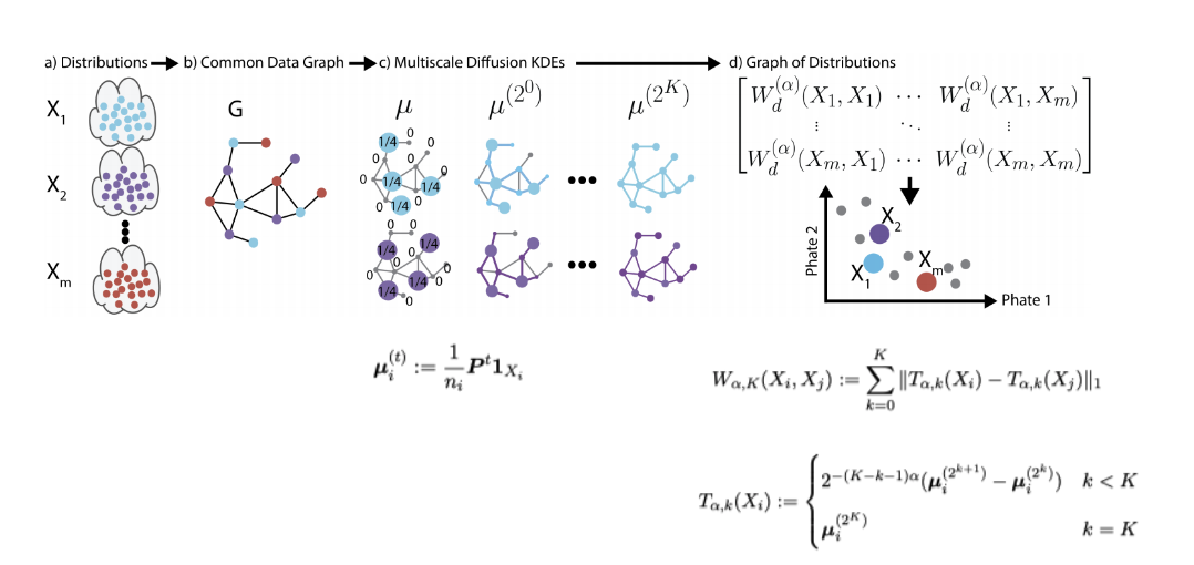
Embeddings using diffusion EMD

Create a higher-level distance matrix using pairwise EMD. Visualize with PHATE to preserve manifold geometry.

Ground manifold distance and EMD: take ground distance as diffusion distance.

Recommended Reading

• Peyre & Cuturi, Computational optimal transport, https://arxiv.org/abs/1803.00567
• Cuturi,Lightspeed computation of optimal transport distances, NeurIPS 2023
• Huguet et al. Geodesic Sinkhorn for fast and accurate optimal transport on manifolds, IEEE MLSP 2023
• Chen et al. Uncovering axes of variation among single-cell cancer specimens, Nature Methods 2020
• Tong et al. Diffusion Earth Mover’s distance and Distribution Embeddings, ICML 2021
• Zapatero, Tong et al. , Trellis tree-based analysis reveals stromal regulation of patient derived organoid drug responses, Cell 2023

9. Riemannian Geometry and ML Applications

Topological space

• Combines a set of points with a topology
• Topology: a colelction of subsets (called open sets) that define the structure of neighborhoods and closeness within the set
• Enables formal analysis of continuity and convergence without relying on a notion of distance (unlike in geometry)

Let $X$ be a set and $\tau$ a family of subsets. $\tau$ is a topology on $X$ if:

• The empty set and $X$ are elements of $\tau$
• $\tau$ closed under unions and finite intersections
• $(X, \tau)$ called a topological space

Topological manifolds

• A manifold is a topological space which is locally Euclidean
• This means each point has a neighborhood which is homeomorphic to an open subset of Euclidean space

$f: X \rightarrow Y$ between two topological spaces is a homeomorphism if:

• it is a bijection
• it is continuous
• inverse image is continuous and maps open sets to open sets (open mapping)

Chart and Atlases

Neigborhood $U$ together with homeomorphism $x: U \rightarrow \R^n$ is a chart. Manifolds which are not homemorphic to $\R^n$ necessarily require more than one chart. The collection of these charts together is an atlas, and the charts allow us to create local coordinate systems for each nbhd and create a tangent basis for it.

We use this idea in manifold learning by using Euclidean distances only to find local neighbors in manifold learning. Recall that we compute pairwise distances when computing kernels. The pointwise kernel function (e.g. Gaussian) eliminates non-local distances.

Importance of neighborhoods: In some manifold learning methods (UMAP, tSNE), there is computation of neighborhoods. The idea is match local neighbors between high and low dimensional embeddings. The idea is that if the charts are matched, then manifold information is carried to low dimensions. This breaks if the manifold is not well sampled (UMAP manifold uniformly sampled assumption).

Differentiable Manifolds

Differentiable manifold a topological manifold with differential structure. A topological manifold can be given a differential structure locally by using the homeomorphisms in its atlas and the standard differential structure on a vector space.

To include a global differential structure on the local coordinate systems induced by the homeomorphisms, their compositions on chart intersections in the atlas must be differentiable functions on the corresponding vector space. Where the domains of charts overlap, the coordinates defined by each chart are required to be differentiable with respect to the coordinates defined by every chart in the atlas. The maps that relate the coordinates defined by the various charts to one another are called transition maps.

The tangent space of a manifold at a specific point is denoted $T_pM$. It is an $n$-dimensional vector space that locally approximates the manifold at that point.

In ML methods where we look at how to move from point to point on a manifold, this assumes some kind of smoothness (differentiability). Therefore, we’re interested in Riemannian geometry.

Rimeannian metric

Given a smooth topological manifold $M$, we introduce geometry to the manifold by prescribing an inner product:

This allows us to define ideas of length and distance:

The metric is a local element of volume or length. It allows us to build up the real volume in small steps. This is exactly what we do when we compute the length of a path on a graph, albeit discretely. When we find a shortest path we are finding the infimum between these paths.

The volume can also be used for density estimation on the manifold: if you have many points in a nbhd, you can divide by the local volume to get local density.

Curvature

Intuition: one way to define curvature in low dimensions is with the osculating circle (a circle that kisses a curve at a point by being tangent to it and have the same curvature as the curve at that point).

In 2-D, there is Gaussian curvature. There are infinitely many curves that pass through any point on a 2d surface. Locally at any point $p$ we can find a unit normal vector $N(p)$ that is perpendicular to the surface at $p$. This is called the Gauss map $N: \R^3 \rightarrow S^2$. We can measure curvature by measuring how fast $N(p)$ changes.

In higher dimesnions, one can look at how a higher dimensional shape is deformed as it moves through the manifold. This requires covariant derivatives, curvature tensor, Ricci tensor, etc.

• Intuitively, Ricci curvature measures how the volume of a small ball or the divergence of geodesics changes in a specific direction on a curved surface, indicating how much the local geometry deviates from the flat EUclidean space.
• Positive Ricci implies convergence of parallal paths (like on a sphere)
• Negative suggests divergence (like hyperbolic)
• A directional average

Gaussian vs Ricci Curvature

• In 2D, the Ricci curvature is the Gaussian curvature
• In higher dimensions, the Gaussian curvature is the sectional curvature of a 2D slice of the manifold
• Ricci curvature is the average of the sectional curvatures of all possible 2D slices that include a given tangent vector.

Curvature on Graphs

Ollivier-Ricci curvature compares distance between points vs. optimal transport of a 1-hop neighborhood.

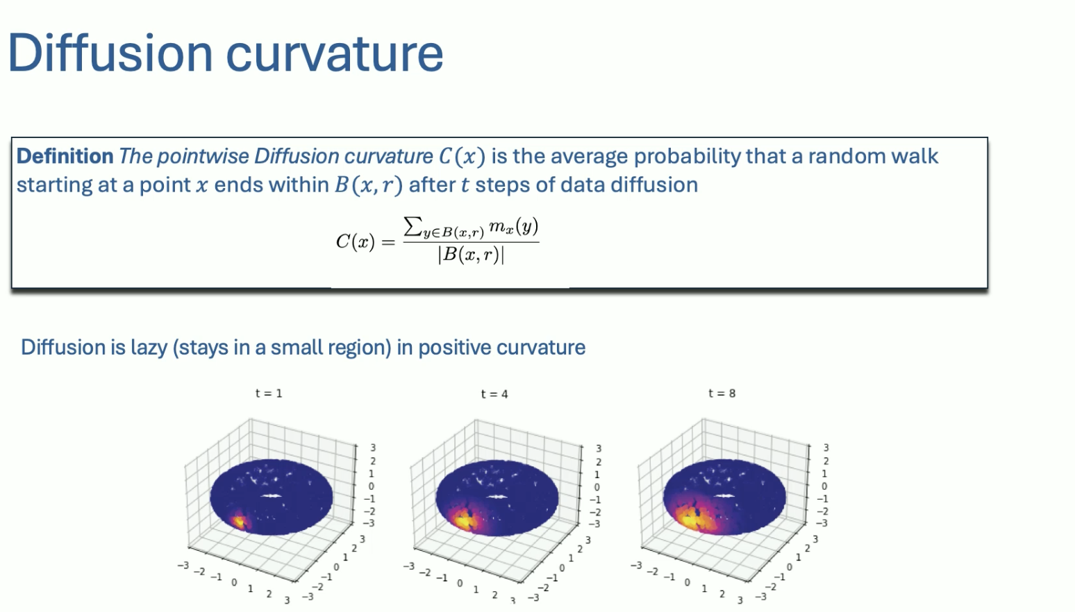
There are other notions of curvatures on graphs, such as the diffusion curvature:

Bishop-Gromov gives us theorems about the volume of balls on Riemannian manifolds.

A comparable volume theorem for diffusion/graphs:

Forman Ricci curvature: useful in GNNs, helps combat “oversquashing” of information or too-tight information bottlenecks. Negative edges can be reinforced to pass additional information.

10. Geometric Manifold Learning

Connecting discrete Laplacian to continuous. Ask when they converge?

Energy in discrete space as

$$f^t L f = \sum_{\text{edges}} w_{ij}(f_i - f_j)^2.$$

Energy in smooth setting, we would want

$$E(f) = < \nabla f, \nabla f > = | \nabla f |^2/$$

Claim that

$$\int_M < \nabla f, \nabla g> d\mu = \int_M f(-\Delta g) d\mu.$$

Pf.

ParseError: KaTeX parse error: Undefined control sequence: \nbala at position 25: …}f \nabla g = <\̲n̲b̲a̲l̲a̲ ̲f, \nabla g> + …

Integrating over manifold on both sides + Stokes’ Theorem,

$$\int_M <\nabla f, \nabla g> d\mu + \int_M f \Delta g d\mu = \int_m \text{div} f \nabla g = 0.$$

We also have similarity in Rayleigh Quotients. E.g., in discrete setting, Rayleigh quotient

$$\min_{|f| = 1} f^T L f = \lambda_2.$$

In smooth,

ParseError: KaTeX parse error: Undefined control sequence: \mun at position 1: \̲m̲u̲n̲ ̲\frac{\int_M | …

Next, connecting diffusions. $L = D-A$ the Laplacian (discrete) and $P =AD^{-1}$ the column normalized random walk operator (same thing as row normalized transpose when we define $P = D^{-1}A$). If $f$ the initial dist (e.g. of heat) on the nodes of graph, $Lf$ represents rate of change of diffusion process over graph and $Pf$ the 1-step transition probabilities. The discrete Laplacian, $L$, the infinitesimal generator of $P$.

Compare this to the heat equation in the smooth setting,

$$\partial_t u(t,x) = \Delta u(t,x).$$

Solution the heat semigroup,

$$P_t f = e^{-t \Delta} f.$$

The Laplacian $\Delta$ the infinitesimal generator of $P_t$:

$$\frac{\partial}{\partial t}P_t \text{ evaluated at t=0 } = - \Delta f.$$

Lastly, convergence–when does discrete Laplacian coincide with smooth Laplacian?

11. Autoencoders and Intro to Generative Models

NN overview, unsupervised learning, representation learning

Autoencoders

• design the AE to it can’t learn to copy the input perfectly
• informational bottleneck
  • new representation is lower dimension / simpler
  • also helps with denoising We call this an undercomplete autoencoder
• hope: training the autoencoder will result in $z$ having useful properties $ $Dim(z) < Dim(x) \implies$ undercomplete AE, forces AE to capture the most salient features of the training data
• AE only approximately copies the input

Linear vs. non-linear AEs

• AEs with only linear layers with no activation function learn PCA
• nonlinear AEs learn a nonlinear dimensionality reduction of the data that can still be decoded
  • e.g., diffusion maps, UMAP are hard to decode
• generalizable (adding new points is easy)

PCA

• finds the directions in input space that explain the most variation, re-represents data by projecting along those directions

PCA as encoder, decoder

• $N$ data vectors $x_i$ with dim $d$, $\bar x$ the sample mean
• want to reduce dimensionality from $k$ to $d$
• sample covariance matrix:

$$\sum = \frac{1}{N} \sum_{i=1}^N (x_i - \bar x)(x_i - \bar x)^T = U \Lambda U^T$$

• $U_k$ contains the first $k$ eigenvectors, giving the directions of most explained variance
• project the data points on this space:
  • encoding $z_i = U_k^T x_i$
  • decoding with $\hat x_i = U_k U_k^T x_i$

Two views of PCA: maximize variance, minimize error

Reconstruction:

• assume data come from $d$-dim vectors where $n$-th vector is $X = (x_1, x_2, ..., x_n)$
• we can represent a point in $d$ dimensional Euclidean space in terms of any $d$ orthogonal vectors, call them $U = (u_1, u_2, ..., u_d)$
• the goal is for $k < d$ find the vectors $U$ such that

$$E = \sum_{i=1}^n ||x - \tilde x||^2$$

is minimized, where $\tilde x$ the projection of $x$ onto the first $k$ components of $U$.

Regularization

Any modification made to a learning algorithm that is intended to reduce its generalization error but not its training error

• e.g., L1 and L2 regularization
• adding noise to inputs
• early stopping
• dropout

An example of bias for simple solutions would be adding # of parameters to the loss function, this penalizes model complexity.

Denoising Autoencoders

• traditional AE minimizes $L(x, g(f(x)))$
• denoising autoencoder minimizes $L(x, g(f(\tilde x)))$
  • $\tilde x$ a corrupted version of $x$
  • denoising AEs learn to undo this corruption
• corruption process $C(\tilde x | x)$ modeled by conditional distribution
• the AE learns a reconstruction distribution $p_{\text{reconstruct}}(x| \tilde x)$ from training pairs $x, \tilde x$

The process:

• sample training example $x$ from training data
• sample corrupted version $\tilde x$ from $C(\tilde x | x)$
• use $(x, \tilde x)$ as a training example for estimating $p_{\text{reconstruct}}(x|\tilde x) = p_{\text{decoder}} (x |z)$
  • $z = f(\tilde x)$ the encoder output $p_{\text{decoder}}$ defined by decoder $g(z)$
• can then perform SGD on negative log likelihood $-\log p_{\text{decoder}} (x|z)$
  • equivalent to doing SGD on $- \E_{x \sim p_{\text{data}}}(x) \E_{\tilde x \sim C(\tilde x | x)} \log p_{\text{decoder}} (x | z = f(\tilde x))$
  • $p_{\text{data}}$ is the training distribution

Denoising autoencoders have been hypothesized to do manifold learning.

Generative models

Usually noise -> neural net -> spit out something like training sample.

Probabilistic interpretation: randomly sampled nosie $X \sim N(\mu, \sigma)$ -> neural net -> sample from training distribution $X \sim P(X)$.

Can we modify a regular autoencoder for generation?

• basic idea: add noise to samples to push them away from the data manifold and then have them pull it back
• for each training sample $X$ define a corruption process $C(\tilde X, X)$ that creates a corrupted sample $\tilde X$
• train a denoising autoencoder to reverse this by using $(X, \tilde X)$ as a training sample

See: generalized denoising autoencoder

Walkback training

• train the neural network to walk back from several steps away
• create longer range corruption processes using the original corruption process
• sample a second step $C(\tilde X^*, \tilde X)$
• add the training sample $(\tilde X^*, \tilde X)$ to the training

This way of training trains the DAE to estimate a conditional probability distribution $P(X|\tilde X)$. Original paper (Bengio 2013) shows that a consistent estimator of $P(X)$ can be recovered by alternating sampling from the corruption process $C(\tilde X, X)$ and the denoising process $P(X | \tilde X)$

However, issues with this approach: data generation process is very slow (like taking slow walk through data), may not span the space, not penalized to generate the distribution.

Variational Autoencoders (VAEs)

Learning latent spaces that allow for sampling, i.e., we want to generate new examples just by sampling in the latent space.

VAEs force the latent vectors to have a roughly unit Gaussian distribution. Generate images by sampling a unit Gaussian and passing it into the decoder.

There exists a tradeoff between accuracy and the unit Gaussian approximation. Build this directly into the loss:

• include a reg term that penalizes the KL divergence between unit Gaussian and the latent vector distribution.
  • note that KL divergence penalizing distributions in latent space from being too far from standard normal encourages every ball to be the same

Recommended reading

• Hinton and Salakhutdinov, Reducing the dimensionality of Data with Neural Networks, Science 2006
• Alain & Bengio, JMLR 2014 What Regularized Auto-Encoders Learn from the Data- Generating Distribution
• Bengio et al. Generalized Denoising Auto-Encoders as Generative Models, NeurIPS 2013
• Kingma & Welling, Autoencoding Variational Bayes, https://arxiv.org/pdf/1312.6114.pdf
• ScVI Lopez et al. Deep generative modeling for single-cell transcriptomics, Nature Methods 2018
• van Dijk et al. Finding Archetypal Spaces using Neural Networks, IEEE Big Data 2019 • Venkat, Youlten et al. AAnet resolves a continuum of spatially-localized cell states to unveil intratumoral heterogeneity, Cancer Discovery 2025

12. Variational Calculus, Pullback Metrics, NeuralFIM

Attach slides; math lecture

13. Probabilistic Methods for Robust and Transparent Machine Learning

Guest lecture

14. Neural ODEs, Flows, and Flow Matching

First part: covering ODEs. ODE deals with one variable and its functions and derivatives. Initial value problem.

• Simple methods for solving ODEs
  • Euler’s method–approximate solution step by step using tangent lines, achieving piecewise linear approximation

Neural ODEs

Resnets are neural networks with skip connections. Neural ODEs paper relates ODEs to Resnets, though it isn’t a super useful analogy.

Neural ODE: a neural network that computes derivatives (Usually NN tries to approx function, neural ODE goes for derivative of that function). The derivative is “parameterized” by a neural network. To compute $F(x,t_1)$ given $F(x,t_0)$ we use an ODE solver.

ODE network layers are calls to ODE solvers. In order to train it, we would have to backpropagate through operations of the ODE solver, but this can be very time consuming even if every operation is differentiable.

To avoid backprop through the ODE solver, they try to approx. the derivative. Approx the SGD using “adjoint sensitivity.”

Adjoint sensitivity method

Suppose we have a loss function whose output is the result of an ODE solver. To optimize $L$ we have to consider its gradient wrt $\theta$, but the parameters in $\theta$ are optimizing the loss function via intermediate variables output by the ODE solver $z(t_0), z(t_1), ...$. We can imagine applying the chain rule to figure this out, which would be weird b/c we have to do this continuously for every value of $t$.

We need a continuous analogue of the chain rule called the sensitivity equation instead. Two DEs: forwards and backwards, used to compute adjoint sensitivity equation, which will approximate derivatives for ODE solver.

Continuous normalizing flows

Neural ODEs can be used to perform population dynamics and not just single entity dynamics. They can do this by using continuous normalizing flows, a continuous extension of normalizing flows. Still trained to maximize the likelihood of the data distribution.

Normalizing flows are a series of invertible simple functions that can be run forwards or backwards. Trained “backwards” from how they operate.

Deep normalizing flows compose the function $f$ into a composition of invertible mappings, starting from a simple noise distribution (which must be easily computable to work).

Maximum likelihood (MLE) training: train a NN to maximize the density it assigns to samples from the data. In the case of normalizing flows, we can compute it exactly using the density of the initial noise distribution, which is Gaussian.

OT Regularized Flows

Optimal transport regularized flows–restricting CNF to optimal transport, helpful for modeling biological and cellular systems. Constrain the derivative network such that they are smoother (penalize $L^2$ norm), this gives rise to optimal transport paths.

Manifold Interpolating Flows

Flow is restricted to be smooth, don’t have to start from noise.

Architecture: autoencoder has PHATE regularization to enforce data embedded via manifold distances.

Train via ODE solver. No longer have observations in cont. time of each cell, so we penalize to match the distribution of the next timepoint. This takes the form of a static optimal transport penalty, or you can use KL divergence. This will give us smooth paths from time point ot time point.

Regularized flow has been shown to yield dynamic optimal transport.

Why would we do MIOFlow? With low-dim PHATE representation, we can flow backwards and look at the decoded trajectories. Can also use Granger causality to understand to infer things like gene regulatory networks (or other causal structure between data).

Flow matching

Neural ODEs (simulation based training) require many integration steps, have high variance gradients. Can we approx OT without Neural ODE?

Use flow matching. If we only care about source to target point, we can assume Euclidean latent space and then the path will be a straight line between source and target points. SO the vector field from the source always points to the target. Flow matching is to regress onto the vector field.

Diffusion based methods can take circuitous paths to the data, whereas flow matching will go right towards it. We can interpret the OT paths as linearly interpolating between a very low variance distribution around a data point and target. OT has been shown to have fast convergence.

15. CNNs and Diffusion Models

Parts:

• CNN review
• VAEs and variational inference
• Diffusion models

Classifier guidance: Some diffusion models take in text or other labels as a prompt, generally accommodated by putting that label in as a conditional label $P(x_0 | y).$ There is also manifold guidance: correcting noise using a denoising autoencoder. The noise then “snaps” onto the data manifold and the diffusion occurs on the data manifold.

• UNet architecture featuring an encoder-decoder framework with skip connections
• Many diffusion models use this to reverse noise, including Stable Diffusion
  • Stable diffusion employs a latent space for the dfifusion, a latent space of a VAE
  • Gaussian noise applied to forward process
  • UNet blocks with residual connections are used to reverse the noise process to recover latent space image representations.

16. Intro to Topological Data Analysis

TDA is interested in the shape, structure, and connectivity of data. Especially suitable for datasets that are high-dimensional, noisy, or incomplete. The central idea is that the shape of data contains valuable information that traditional statistical methods might miss. One challenge with the extracted topological and geometric information is trying to incorporate it in a differentiable framework.

A core TDA concept is using individual data points to build a “continuous” shape that approximates the data. This follows a pipeline:

• Input data: data is typically assumed to be a finite set of points, i.e., a point cloud in a metric space.
• Build a shape: A geometric structure called a simplicial complex is constructed from the point cloud by connecting nearby points with edges, triangles, and higher-dimensional shapes.
• Analyze the shape: look at the topological features of this shape, such as connected components (clusters), loops (holes), and voids (cavities). Extract these and quantify them using methods like persistent homology.

Datasets are usually finite sets of discrete observations, do not directly reveal any topological information. A natural way to highlight some topological structure out of this data is to “connect” it with neighbors that are close, quantified via metric space. TDA considers data sets as discrete metric spaces or samples from continuous metric spaces.

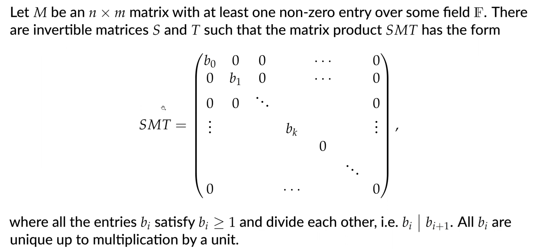
Simplices

Given a set $X= \{x_0, x_1, ..., x_k\} \in \R^k$ of $k+1$ affinely independent points, the $k$-dimensional simplex $\sigma = [x_0, x_1, ..., x_k]$ is the convex hull of $X$. The points of $X$ are the vertices of the simplex. Simplices spanned by subsets $S \subset X$ are called the faces of $\sigma$.

A simplicial complex $K \in \R^d$ is a collection of simplices such that:

• any face of a simplex in $K$ is also a simplex in $K$
• any non-empty intersection of two simplices $\sigma_1, \sigma_2 \in K$ is a face of both.

Abstract vs Geometric Simplicial Complexes: $K$ is fully characterized by the combinatorial description of a collection of simplices satisfying some incidence rules. We can define simplicial complexes with no reference to geometry:

• Given a set $V$, an abstract simplicial complex with vertex set $V$ is a set $\tilde K$ of finite subsets of $V$ such that for any set $\sigma \in \tilde K$, any subset $\tau \in \sigma$ is also in $\tilde K.$
• The subsets of $\tilde K$ are called the faces of $\tilde K$. The dimensionality of this simplicial complex is cardinality minus 1.

The combinatorial description of any geometric simplicial $K$ gives rise to an abstract simplicial complex $K$. Conversely, we can associate an abstract simplical complex $\tilde K$ a topological space $|\tilde K|$ such that if $K$ is a geometric complex whose combinatorial description is the same as $\tilde K$, then the underlying space of $K$ is homeomorphic to $|\tilde K|.$ Such a $K$ is called a geometric realization of $|\tilde K|$.

Abstract simplicial complexes can be seen as topological spaces and geometric complexes can be seen as geometric realizations of their underlying combinatorial structure.

Therefore, we can consider simplicial complexes simultaneously as combinatorial objects for effective computation and as topological spaces from which we can infer topological properties.

Building simplicial complexes from data

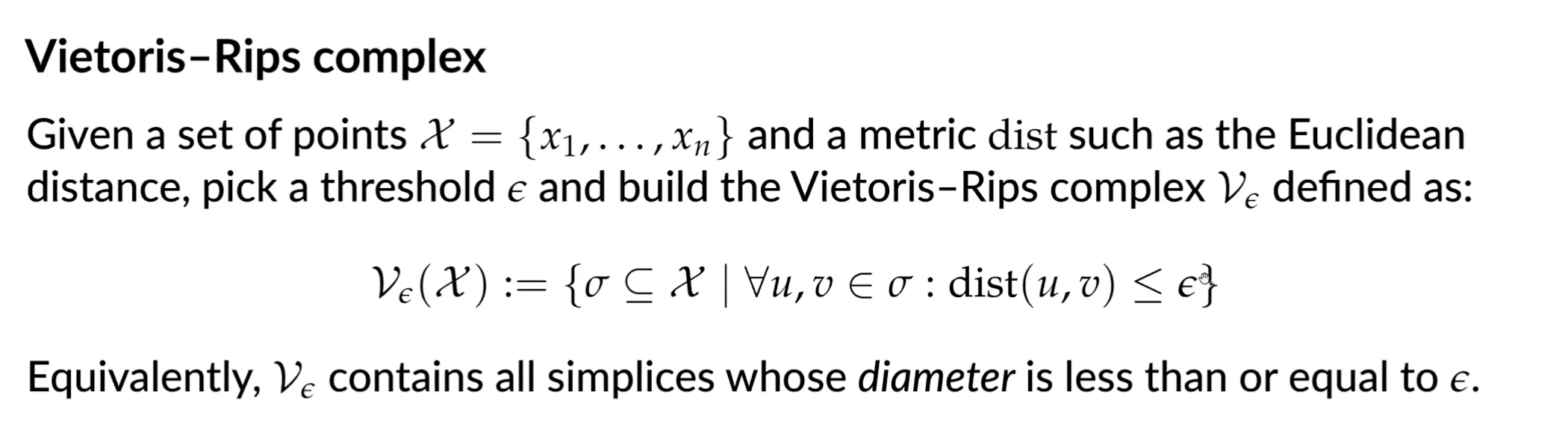
Given a dataset, there are many ways of building a simplicial complex. A common method is the Vietoris-Rips complex:

• Assume we are given a set of points $X$ in a metric space $M$ and a real number $\alpha \geq 0$. Then the VR complex, denotes $\text{Rips}_\alpha(X),$ is the set of simplices $\sigma = [x_0, ..., x_k]$ such that $d(x_i, x_j) \leq \alpha$ for all $(i,j).$

It follows immediately from the definition that this is an abstract simplicial complex. However, in general, even when $X$ is a finite subset of $\R^d$, $\text{Rips}(X)$ does not admit a geometric realization in $\R^d$, and in particular, it can be of dimension higher than $d$.

The Cech complex $\text{Cech}_\alpha(X)$ is the set of simplices $\sigma = [x_0, x_1, ..., x_k]$ such that the $K+1$ closed balls $B(x_i, \alpha)$ have nonempty intersections

$$\cap_{i=0}^k B(x_i, \alpha) \neq \emptyset.$$

This is different from the VR complex in that unless balls centered at $x_1, x_2, x_3$ have a 3-way intersection, there is no triangle formed in a Cech complex.

Nerves

Given a cover of a dataset, its nerve provides a compact and global combinatorial description of the relationship between these sets through their intersection patterns.

Nerve theorem: Given a cover $U = (U_i)_{i\in I}$ of $M$, the nerve of $U$ is the abstract simplicial complex $C(U)$ whose vertices are the $U_i$’s and such that $\sigma = [U_{i0}, ..., U_{ik}] \in C(U)$ if and only if $\cap_{j=0}^k U_{ij} \neq \emptyset.$

Using the nerve of covers as a way to summarize, visualize, and explore data is a natural idea first proposed in Singh (2007), giving rise to the Mapper algorithm.

Mapper algorithm used to convert complex, high-dim data into a simplified and understandable graphical representation based on the idea of a nerve:

• Filter data into a lower dim: a filter function projects the data to a lower-dim space, typically a 1 or 2-dim line.
• Divide the filter data: the lower-dim space is divided into several overlapping intervals or “bins”
• Cluster data within each bin: the algorithm “pulls back” the bins to the original, high-dim dataset. For each bin, a clustering alg. is run on all the data points that fall within it. The resulting clusters become the nodes/vertices in the Mapper graph
• Create the graph: an edge is drawn between any wo nodes if their corresponding clusters share any data points. This process connects the clusters to represent the overall topological structure of the data.

Choice of filter function will affect the results. Common ones include density estimates, PC coordinates, centrality measures, and distances from root.

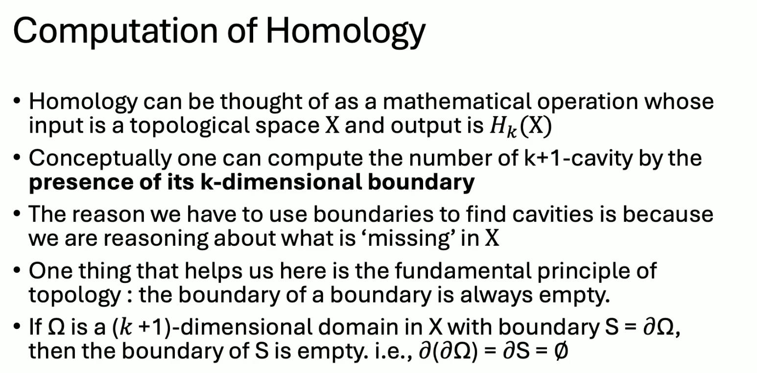
Homology

• Homology is a classical concept in algebraic topology providing a powerful tool to formalize and handle the notion of topological features of a topological space or of a simplicial complex in an algebraic way.
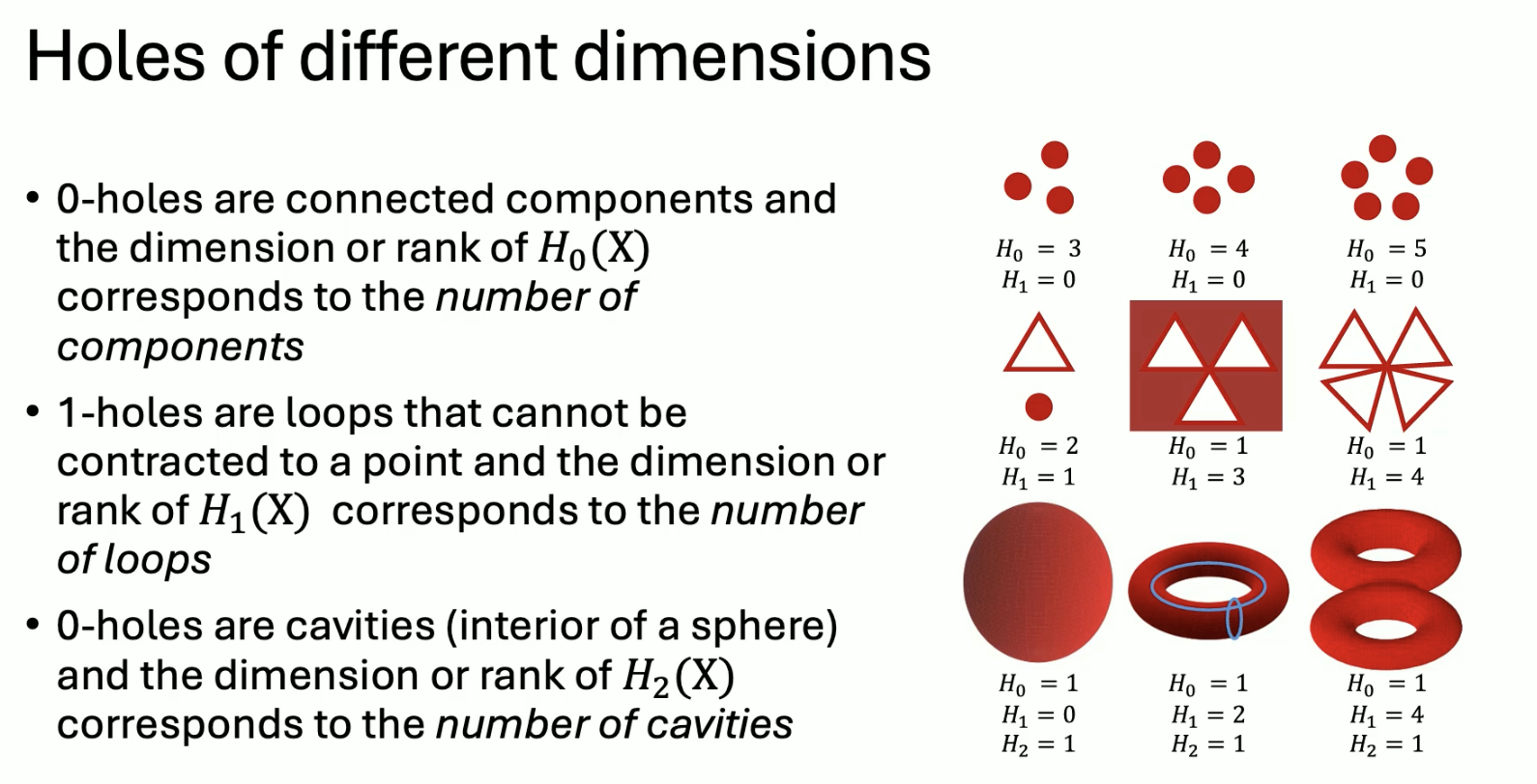
• For any dimension k, the k-dimensional “holes” are represented by a vector space $H_k$ whose dimension is intuitively the number of such independent features
  • For example, the 0-dimensional homology group $H_0$ represents the connected components of the complex
  • The 1-dimensional homology group $H_1$ represents the 1-dimensional loops
  • The 2-dimensional homology group $H_2$ represents the 2-dimensional cavities

17. TDA Guest Lecture

Computational topology: a subfield of algebraic topology that actually tries to compute things on a computer.

Think: why is a cube more similar to a sphere than a torus? The hole in the middle? How can we calculate this? Which qualities of the sphere make it different from the torus?

One idea: Betti numbers. $\beta_0, \beta_1, \beta_1$ measures connected components, tunnels, and voids in that order.

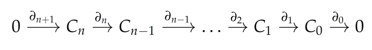
Chain groups

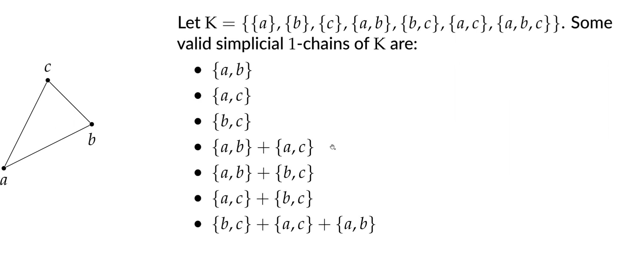
Given a simplicial complex $K$, the $p$-th chain group $C_p$ of $K$ consists of all combinations of $p$ simplices in the complex.

Coefficients are in $\mathbb{Z}_2$, so all elements of $C_p$ are of the form $\sum_j \sigma_j$ for $\sigma_j \in K$. The group operation is addition with $\mathbb{Z}_2$ coefficients.

Boundary homomorphism

Given a simplicial complex $K$, the $p$-th boundary homomorphism is a function that assigns each simplex $\sigma = \{v_0, ... v_p\} \in K$ to its boundary:

$$\partial_p \sigma = \sum_i \{v_0, ..., \hat v_i, ..., v_k\}$$

where $\hat v_i$ indicates the set does not contain the $i$-th vertex. The function $\partial_p : C_p \rightarrow C_{p-1}$ is thus a homomorphism between the chain groups.

For all $p$, we have $\partial_{p-1} \circ \partial_p = 0$: boundaries do not have a boundary themselves. This leads to the chain complex.

The cycle group ParseError: KaTeX parse error: Undefined control sequence: \partal at position 18: …p = \text{ker} \̲p̲a̲r̲t̲a̲l̲_p and the boundary group $B_p = \text{im} \partial_{p+1}.$

$B_p$ is a subgroup of $Z_p$.

Homology groups and Betti numbers

The $p$-th homology group $H_p$ is a quotient group, defined by removing cycles that are boundaries from a higher dimension:

$$H_p = Z_p / B_p = \text{ker} \partial_p / \text{im} \partial_{p+1}.$$

The $p$-th Betti number is calculated as

$$\beta_p = \text{rank}H_p.$$

Intuition: Calculate all boundaries, remove the boundaries that come from a higher-dim object, and count what is left.

Homology calculations in practice use Smith normal form:

Vietoris-Rips Complex

Issues with this approach: how to pick the right $\epsilon$? Also may be computationally inefficient: matrix reduction has to be performed for every simplicial complex.

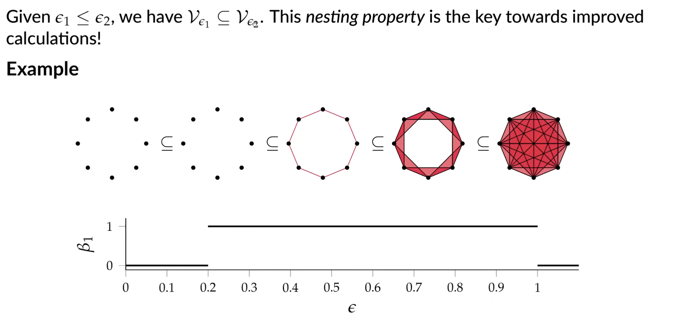
The fix: calculate topological features for all possible scales. How is this any better?

By going through all the scales and tracking topological features, we can see the “destruction” and “creation” of features. We will then be able to identify at what scales features appear and disappear.

This works because VR complex has nesting property.

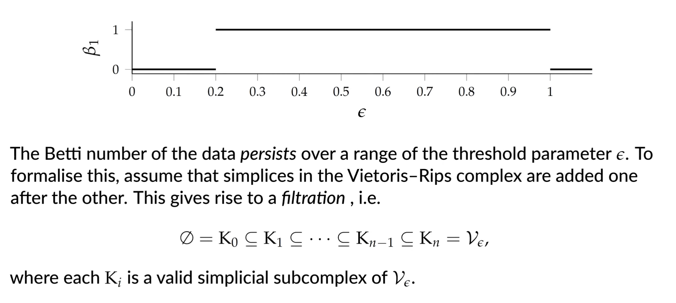
Persistent Hommology Group

Given two indices $i \leq j,$ the $p$-th persistent homology group $H_p^{i,j}$ is defined as

$$H_p^{i,j} := Z_p(K_i) / (B_p(K_j) \cap Z_p(K_i)),$$

which contains all the homology classes of $K_i$ that are still present in $K_j$.

We can calulate a new set of homology groups alongside the filtration and assign a ‘duration’ to each topological feature.

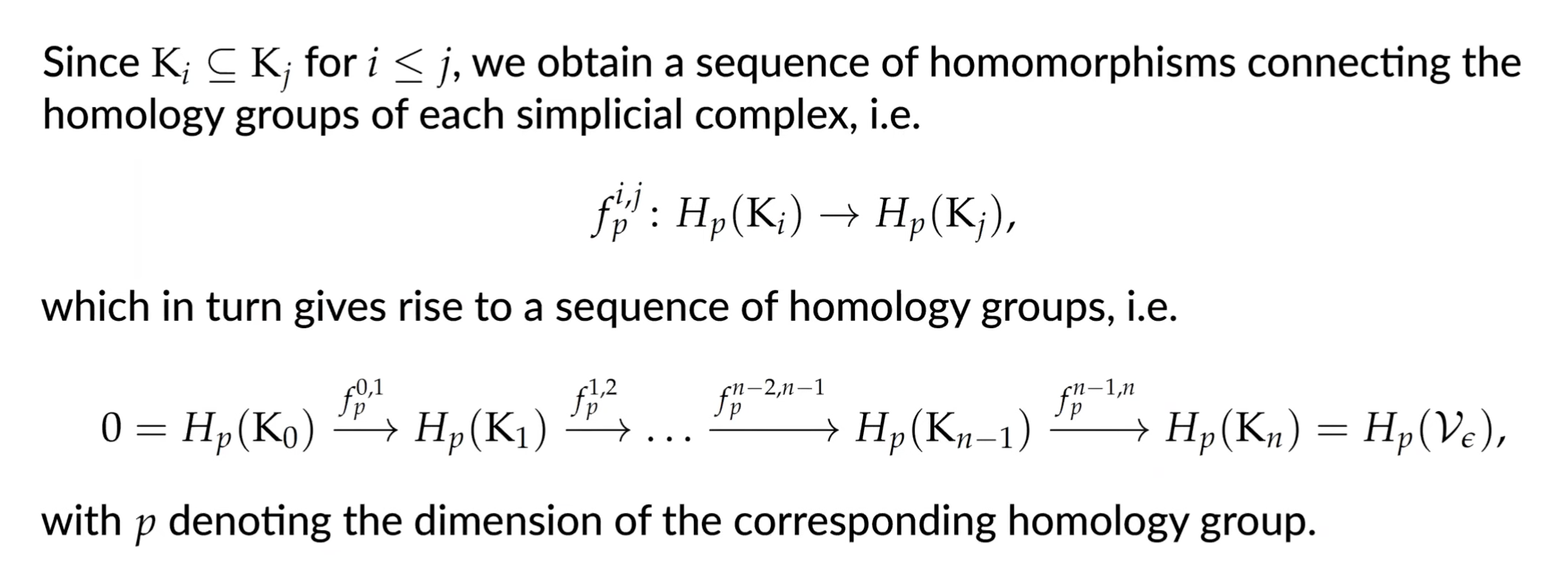
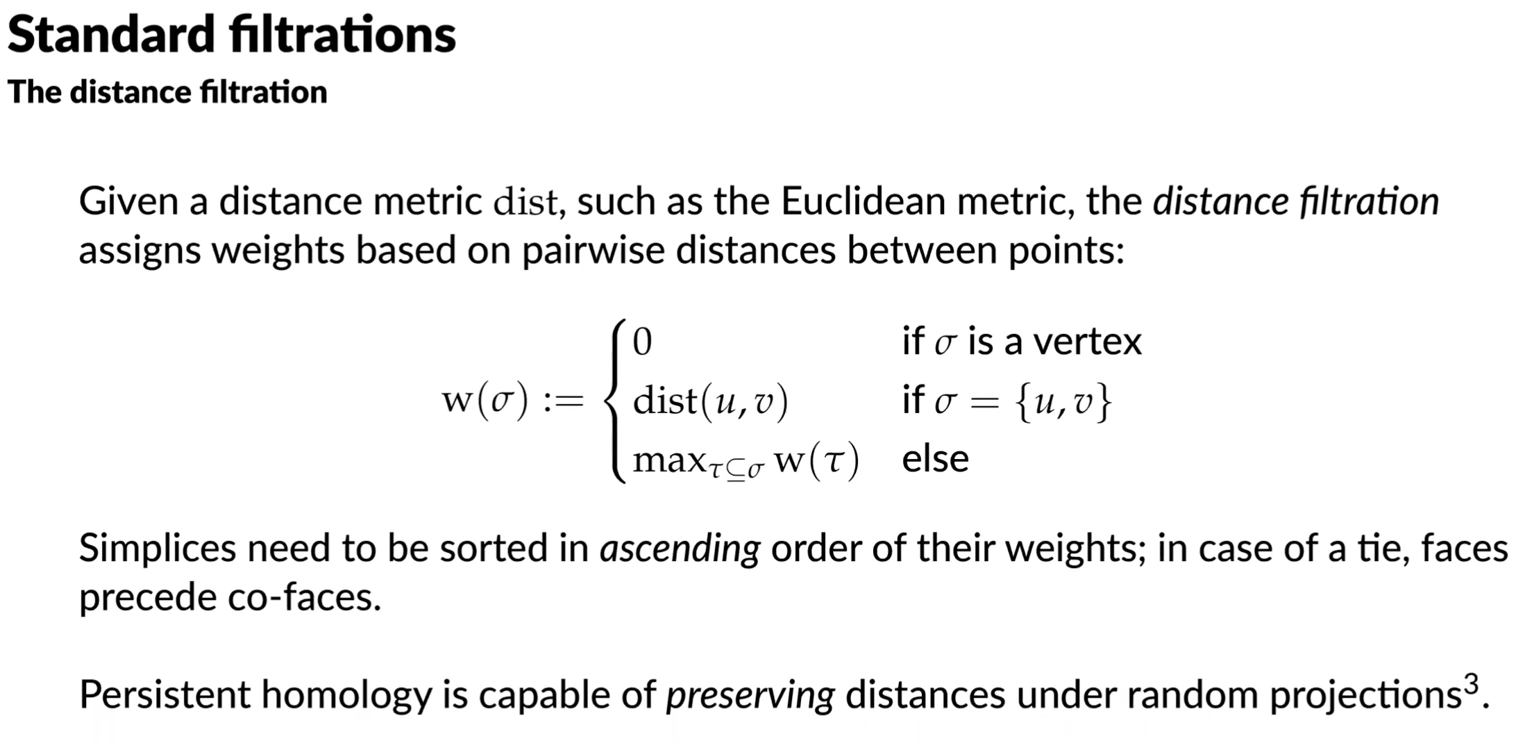
Standard filtrations

Given boundary matrix, we can reduce it. We can examine a reduced boundary matrix for topological information:

• if column $i$ is empty, then $\sigma_i$ is a positive simplex that creates a topological feature
• if column $j$ is non empty with low(j) = k, then $\sigma_j$ is a negative simplex that destroys the topological feature created by $\sigma_k$

Tracking topological features

Given a topological feature with associated simplicial complexes $K_i$ and $K_j$, store the point $(w(i), w(j))$ in a persistence diagram. If the feature is never destroyed, we assign it a weight of $\infty.$

18. Homology in ML

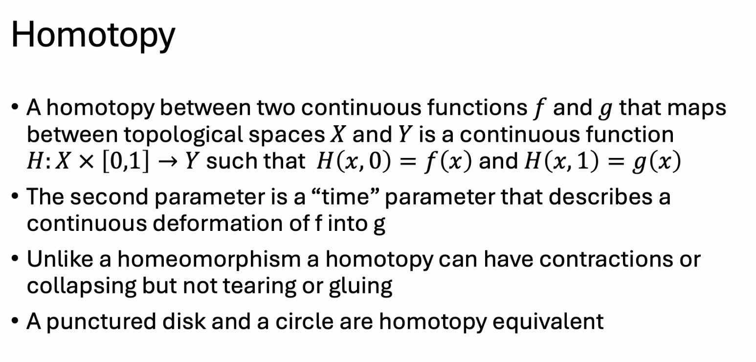
Homotopy: a homeomorphism where you can “contract” things. Involves a cross product with time parameter in domain.

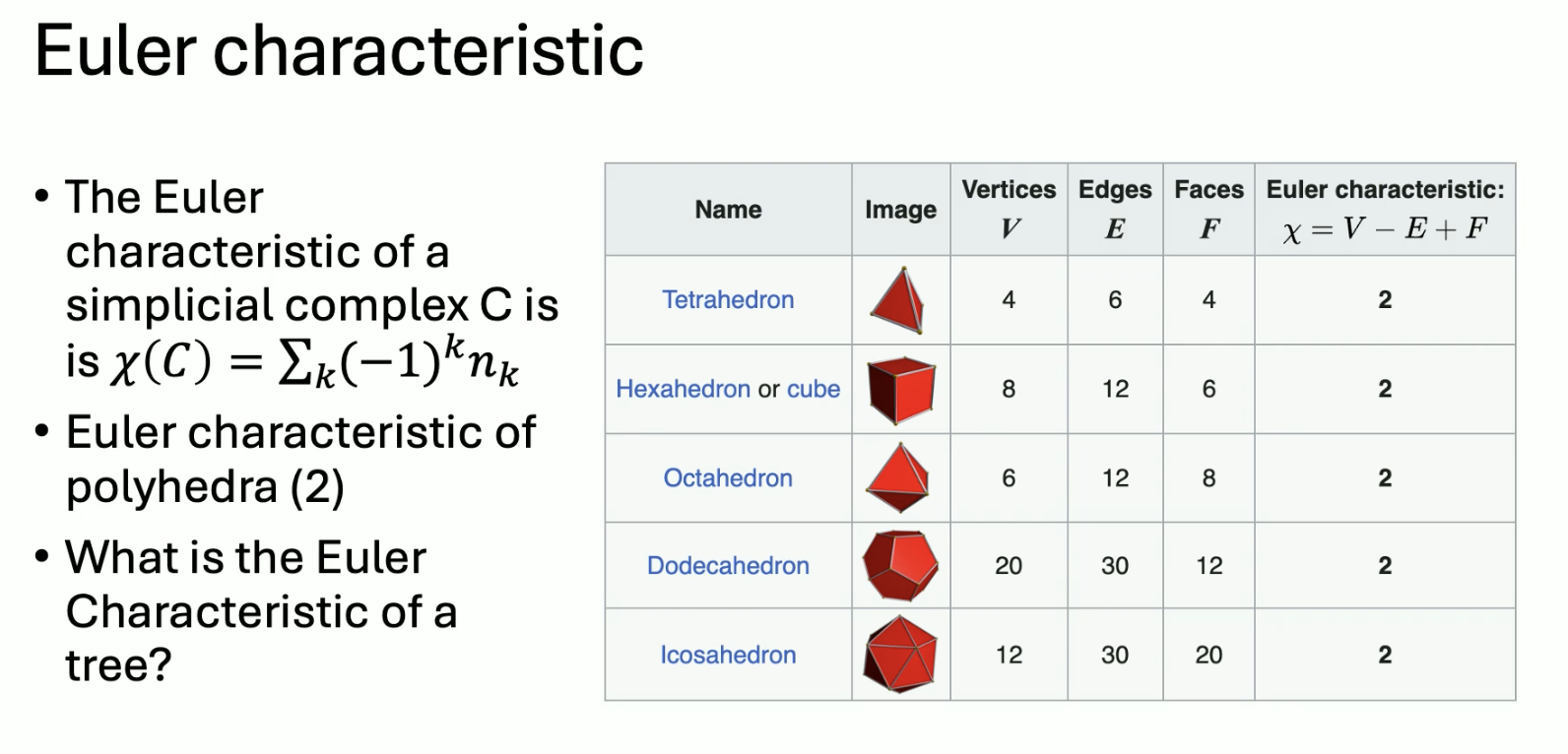
Topological invariant: a property of a mathematical object that remains unchanged under a homemorphism. An example is the Euler characteristic:

Another invariant is homology:

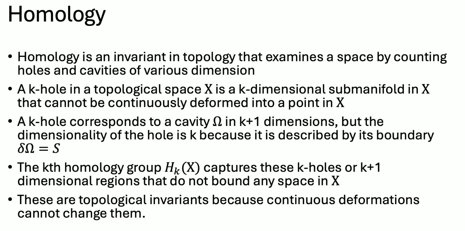
Thus to compute cavities:

• Find all k-dim submanifolds with no boundary (k cycles)
• Eliminate those that bound a domain (k boundaries)

We can repeat this in a lower dimension.

Chains

A k simplex is represented by listing its vertices. We call the union of k simplices a k subcomplex of $X$. The group of $k$ chains, or the $k$-th chaing roup, is the group of all possible k-dimensional subcomplexes you can have.

To identify $k$ holes in the simplicial complex, we have to identify $k$ subcomplexes that have no boundary. The boundary operator maps $k$ chains to their $k-1$ dimensional boundaries

$$\delta_k: C_k(X) \rightarrow C_{k-1}(X).$$

The boundary operator is linear and can therefore be represented by a matrix.

From the chain group, we can get the $k$th cycle group $Z_k(X),$ the kernel of the boundary operator. This includes all $k$ chains that map to 0.

Of all the boundaryless k subcomplexes we find, we need to eliminate the ones that bound a $k+1$ subcomplex. For this we look at the image of the boundary map on $C_{k+1}(X).$ The k boundary is

$$B_k(X) = \delta_k C_{k+1}(X) \subset C_k(X).$$

Homology group

• k chains $C_k(X)$ represent all k subcomplexes in $X$
• k cycles $Z_k(X) \subset C_k(X)$ represent k subcomplexes with no boundary
• $B_k (X) \subset Z_k(X)$ represent $k$ subcomplexes which bound a $(k+1)$ domain in $X$
• to identify $k$ holes, consider all $k$ cycles, and among them, eliminate all $k$ boundaries in $X$ because they are not real cavities
• the $k$-th homology group is the quotient group:

$$H_k = Z_k(X) / B_k(X).$$

Persistence homology in ML constructs a nested sequence of simplicial complexes called a filtration. This tracks the birth and death of k-holes, and we can store this infomration in a persistence diagram.

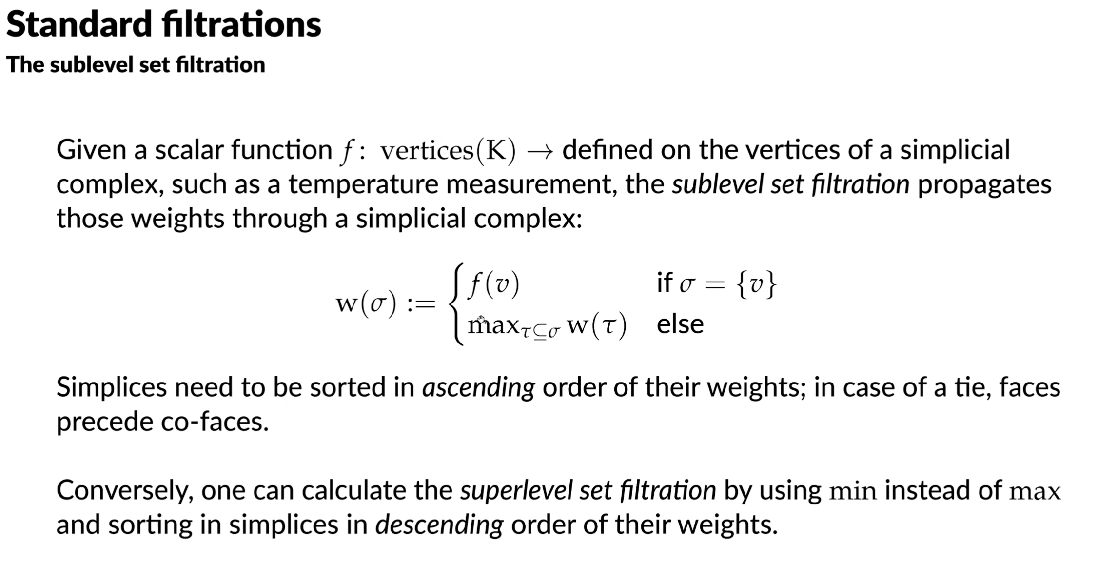
Sublevel set filtration

Thresholding values on objects, e.g. imagine we have grayscale images:

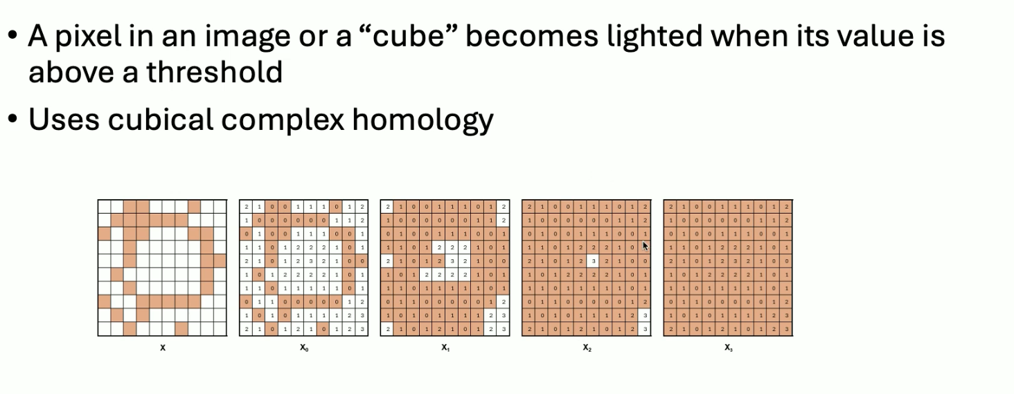
This filtration can be used when we already have a geometrically structured object (e.g. images). This uses cubical complexes as opposed to simplicial complexes.

In cubical complexes, vertices and edges correspond to the same, but triangles now correspond to squares, and tetrahedra correspond to cubes.

19. (20?) Various Filtrations for Graphs and Point Clouds

Filtrations:

• VR filtration
• sub level set filtration
• graph filtrations
  • node functions, edge functions
  • vr filtration based on graph dist
• diffusion condensation filtration and PHATE
• multiparameter filtrations
• zigzag persistence

Filtrations through node and edge functions:

• node functions could include degree, centrality, heat kernel
• edge functions could include edge weights, OR curvature

Centrality: assigns a ranking to nodes based on their network position. Diff types: betweenness centrality (how many times a nodes appears in shortest path b.t. two other nodes), eigencentrality (measures a node’s influence on other nodes).

Eigenvector centrality: Let there be a graph $G= (V,E)$ with adj. matrix $A(i,j)$. The relative centrality score of vertext $i$ is $c(i) = \sum_j A(i,j) c(j).$ Rewriting, we get $AC = \lambda c$; this can be any eigenvector. With the additional constraint that $c(i) > 0,$ we get that it must be the largest eigenvector of $A$ based on Perron Frobenius norm.

Graph filtrations

Graph filtrations based on node-edge functions create an ordering of nodes or edges. Based on the threshold of the function, subgraphs “appear” in a nested fashion.

Graph distance filtration: converts a graph to a point cloud, compute pairwise graph (geodesic distances) b.t. points. Then compute VR complex.

Condensation filtration [ add image ]

Convergence

Application of a positive diffusion operator to a datapoint makes it a convex combination of the points in the dataset, and thus it goes into the interior of the current data convex hull. The convex hull shrinks at a rate proportional to $\partial$ which is the smallest value in the kernel.

Multiscale PHATE: PHATE on frozen diffusion condensation clusters.

Multiparameter persistence

For original persistence homology, the term single persistence is applied because we filter the data in just one direction $K_1 \subset K_2 \subset ... \subset K_n.$ But there are several ways to expand a single filtration into multifiltration to get finer information on the topological patterns.

Multifiltration: multiparameter filtration refers to sweeping through two variables. The result is a bifiltration with columns and rows nested.

Multifiltration in a graph: Use two different node/edge functions $f,g$. These induce a multifiltration $F: V \rightarrow \R^2$ where $F(v) = (f(v), g(v)).$

Multifiltration in a point cloud: consider using a radius $r_i$ and a density estimate at each point $p_i.$ One is VR filtration, and the other is a level-set filtration. At each threshold of the density, we can construct a complete Rips filtration.

Vectorizing multifiltrations: birth and death are hard to compute; the two variables may only form a partial ordering. Multiparameter Betti numbers are an option, as well as sliced persistence diagrams (examine a series of slices as normal persistence diagrams).

Zigzag persistence: Persistence homology for time varying point clouds or graphs. Instead of going in the same direction for filtration, it zig zags (goes back in forth) in directionality. It uses intersections to create the intermediate steps.

Ordinal partition networks:

• create an m-interval windows
• each interval has a value of the filter function, rank order the intervals in the window
• each window represents one of $m!$ permutations of $m$ values
• create a graph with nodes representing permutations
• edges represent transitions between permutations

Given time series $x=[x_0, x_1, ..., x_n]$ for a sequence of times $x=[t_0, t_1, ..., t_n],$ the ordinal partition network is defined by all generating permutations of length $m$ (of which there are $m!$), and then adding edges when they chronologically follow one another.

• keep track of edges added as time flows forward
• this creates a series of temporal graphs
• these are featurized using zigzag persistence.

20. Another guest lecture… topological deep learning

An objection to point cloud -> persistent homology -> featurized input to machine learning pipeline is that it degrades topology to just a set of handcrafted features.

A way to “reverse” this pipeline? How can we learn suitable representations?

Toopological autoencoders, motivation: classic AE struggles to find a representation which preserves multiple scales all at once. If you have data which appears at different scales (e.g., nested spheres), it’s hard to craft a low-dim representation that preserves all that information.

TAE: input data + reconstruction gives reconstruction loss. Topological info of input data AND latent data is compared to give topological loss. The topological loss term serves as regularization.

Why this works: let $X$ be point cloud of size $n$ and $X^m$ be one subsample of $X$ of size $m$ sampled without replacement. We can bound the probability of the persistence diagrams of $X^m$ exceeding at threshold in terms of the bottleneck distance as

$$P(W_\infty (D^X, D^{X^m}) > \epsilon) \leq P(\text{dist}_H (X, X^m) > 2 \epsilon),$$

where $\text{dist}_H$ is the Hausdorff distance. So mini batches are topologically close if the subsampling is not too coarse.

Gradient calculation: everything is based on distances. Every point in the persistence diagram can be mapped to one entry in the distance matrix. Each entry is a distance, so it can be changed during training.

Loss term is bidirectional: how much topo info is preserved going from input to latent + the reverse.

Topology-driven graph learning

Main issue: two graphs can have different numbers of vertices. So we need a vectorized representation $f: G \rightarrow \R^d$ of graphs. Such a representation $f$ needs to be permutation invariant.

Message passing is incapable of capturing large-scale cycles in a graph (and other things, eg oversmoothing problems). In topological graph NN, use a node map $\phi: \R^d \rightarrow \R^k$ to create $k$ different filtrations of the graph. Create persistence diagrams from these graphs, and use a coordinatisation function $\psi$ to create compatible representations of the node attributes. Then aggregate for outputs.

Choosing $\phi, \psi$? The node map can be realized using a neural network. The coordinatisation function can be realized using any vectorization of persistence diagrams, though a differentiable coordinatisation function is most effective.

Sheaves

Let $G$ be a finite, undirected graph with fixed orientation on each edge. Cellular sheaves on $G$: a finite dimensional real vector space, known as the stalk, $F(v)$ for each $v$ vertex and $F(e)$ for each edge. For each incident vertex edge pair, we have a linear restriction map $Fv$ (funky symbol) $e: F(v) \rightarrow F(e).$